부록 L — R-실습: 관측값에 대한 진단

L.1 교과서 예제 3.8

자료 usedcars 에 대한 잔차 분석 (예제 3.8, 예제 5.3) 입니다.

먼저 자료 usedcars 에서 주어진 모든 설명변수를 사용하여 중회귀모형을 적합해 봅니다.

usedcars.lm <- lm(price ~ year + mileage + cc + automatic, usedcars)
summary(usedcars.lm)


Call:
lm(formula = price ~ year + mileage + cc + automatic, data = usedcars)

Residuals:
    Min      1Q  Median      3Q     Max 
-177.35  -63.91   -0.99   70.34  212.69 

Coefficients:
              Estimate Std. Error t value Pr(>|t|)    
(Intercept)  5.253e+02  3.998e+02   1.314 0.200823    
year        -5.800e+00  9.283e-01  -6.247 1.55e-06 ***
mileage     -2.263e-03  7.211e-04  -3.138 0.004324 ** 
cc           3.888e-01  2.022e-01   1.923 0.065958 .  
automatic    1.653e+02  3.986e+01   4.147 0.000339 ***
---
Signif. codes:  0 '***' 0.001 '**' 0.01 '*' 0.05 '.' 0.1 ' ' 1

Residual standard error: 101.1 on 25 degrees of freedom
Multiple R-squared:  0.9045,    Adjusted R-squared:  0.8892 
F-statistic: 59.21 on 4 and 25 DF,  p-value: 2.184e-12

L.1.1 잔차그림

R 에서는 plot 함수를 이용하여 기본적인 잔차그림을 그릴 수 있습니다.

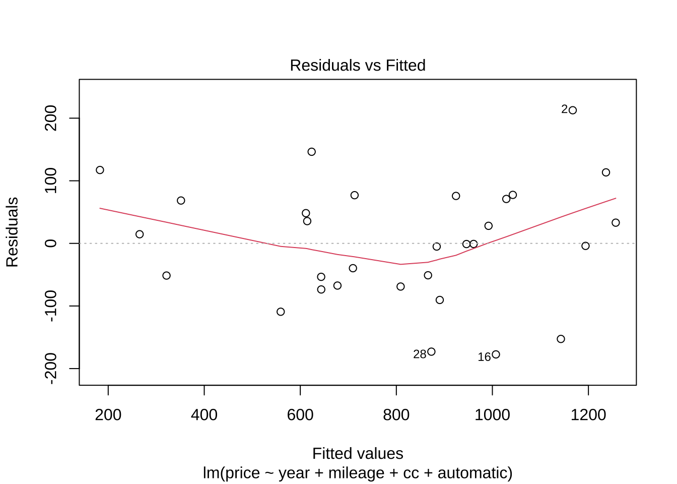
그림 Reidual vs Fitted 는
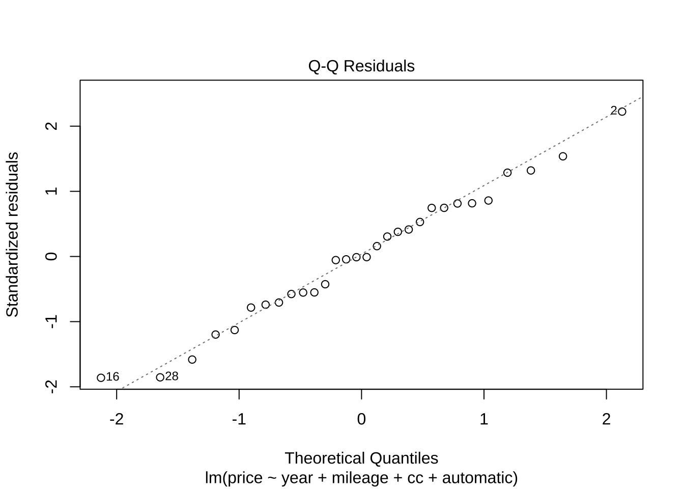
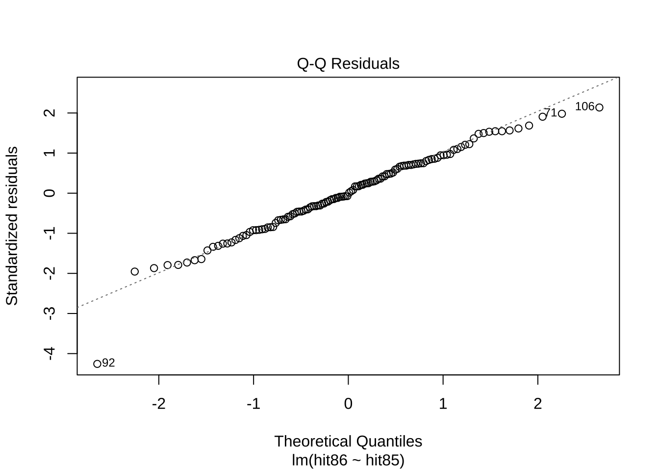
그림 Normal Q-Q 는 잔차가 정규분포를 따르는지를 확인하는 그림이다.
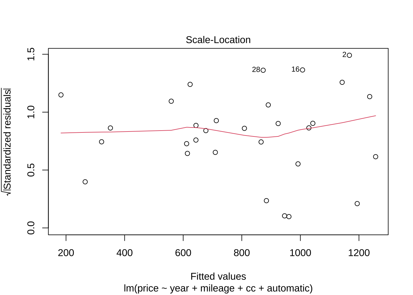
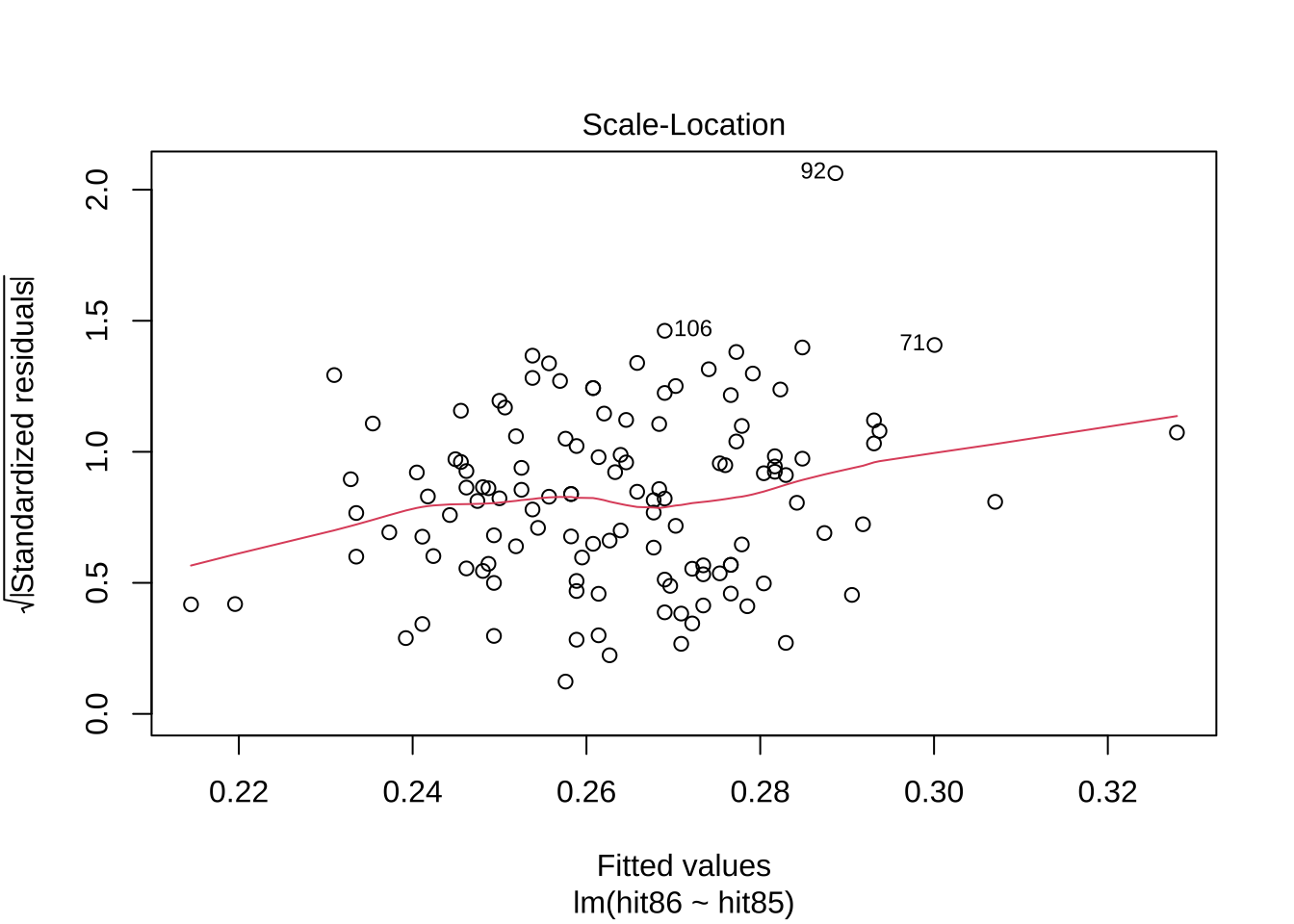
그림 Scale-Location 은 예측값 \(\hat y_i\) 에 대한 표준화된 잔차 \(r_i/\sqrt{1-h_{ii}}\) 를 그린 것이다.

잔차 대 예측값(Residuals vs Fitted)

이 그래프는 등분산성(homoscedasticity)과 선형성 가정을 확인하는 데 도움이 된다.
각 예측값 \(\hat y_i\) 에 대한 잔차 \(r_i\) 를 그린 것이다.
이상적으로는, 잔차들이 수평축(0-라인) 주변에 무작위로 흩어져 있어야 하며, 이는 관계가 선형이고 오류 항의 분산이 일정함을 나타낸다.

정규 Q-Q(Quantile-Quantile)

정규 Q-Q 그래프는 잔차의 정규성을 확인하는 데 사용된다.
점들이 제공된 직선을 따라 배치되어야 이상적이며, 이는 잔차가 정규 분포에 가깝다는 것을 나타낸다.
주어진 선으로부터의 이탈은 정규성으로부터의 벗어남을 나타낸다.

스케일-위치(Scale-Location) 또는 스프레드-위치(Spread-Location)

잔차 대 예측값 그래프와 유사하게, 스케일-위치 그래프는 잔차의 퍼진 정도를 보여주므로 등분산성을 확인하는 데 사용된다.
스케일-위치 그래프(또는 스프레드-위치 그래프)의 y축은 일반적으로 표준화된 잔차 절대값 의 제곱근을 나타낸다.
잔차 절대값 의 제곱근을 보여주는 것은 잔차의 분산을 안정화하는 데 도움을 주어, 이질적 분산(등분산성이 아닌)의 패턴을 시각적으로 더 쉽게 식별할 수 있게 한다.
점들이 대략적으로 수평선을 이루고 균등하게 퍼져 있어야 등분산성의 가정이 적합하다고 판단된다.

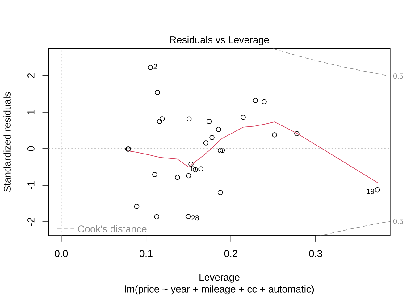
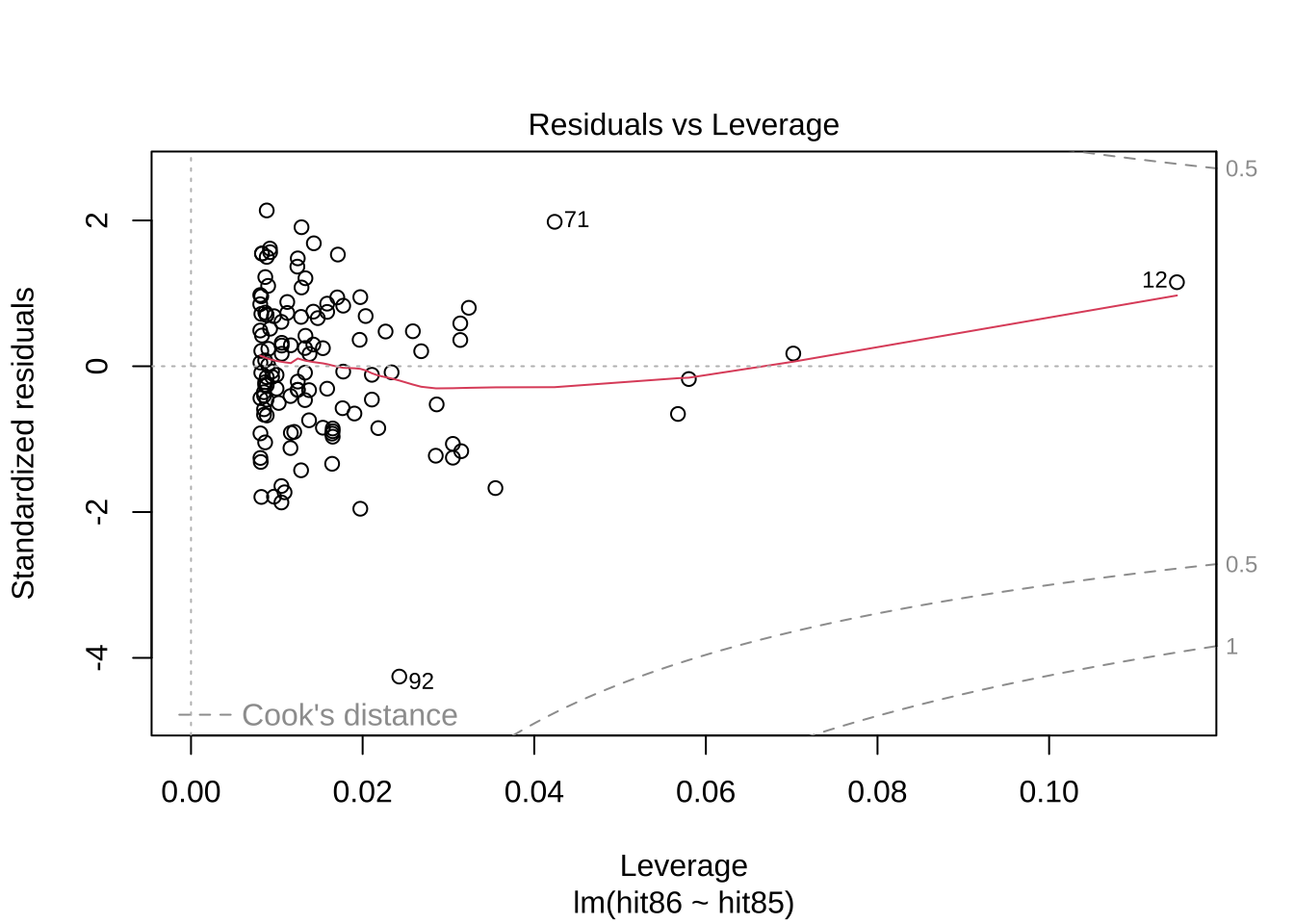
잔차 대 지렛값(Residuals vs Leverage)

이 그래프는 회귀선에 영향을 줄 수 있는 영향력 있는 관찰값을 식별하는 데 도움이 된다.
높은 지렛값와 큰 잔차를 가진 관찰값(이상치)을 잘 파악할 수 있도록 만들어진 그림이다.
이 그래프에서는 다음과 같은 통계량들이 제시되는 것에 유의하자.
- x축: 지렛값(leverage Values, \(h_{ii}\))
- y축: 표준화된 잔차(Standardized Residuals)
- 등고선: Cook’s Distance

plot(usedcars.lm)

L.1.2 잔차

다음과 같은 함수를 통하여 다양한 잔차들와 지렛값을 구할 수 있다.

resid_inter <- rstandard(usedcars.lm)  # internally studentized residual - 내표준화 잔차
resid_exter <- rstudent(usedcars.lm)   # externally studentized residual - 외표준화 잔차
hatval <- hatvalues(usedcars.lm)       # leverage value - 지렛값
data.frame(resid_inter , resid_exter, hatval)

    resid_inter  resid_exter     hatval
1   0.859118727  0.854468915 0.21455013
2   2.223678962  2.432560486 0.10501551
3  -0.553417436 -0.545588388 0.15599165
4  -0.044084943 -0.043195925 0.18996253
5  -0.576180936 -0.568325835 0.15814304
6   0.816421059  0.810807796 0.11903880
7  -0.551399974 -0.543574935 0.16470220
8  -1.198080391 -1.209098031 0.18743332
9   0.378399054  0.371820157 0.25147525
10  0.745189938  0.738380670 0.17431785
11 -0.010873657 -0.010653990 0.07847932
12  1.537452127  1.583088042 0.11334881
13 -0.706665346 -0.699408397 0.11029244
14  1.286252868  1.304157036 0.23928783
15  0.305838319  0.300221293 0.17774944
16 -1.862061057 -1.965848316 0.11253640
17 -0.425962246 -0.418878889 0.15297508
18 -1.582023043 -1.634007936 0.08908012
19 -1.128902196 -1.135412108 0.37287989
20  0.746526192  0.739734875 0.11591279
21 -0.739861832 -0.732982630 0.15005336
22 -0.783820912 -0.777598695 0.13701582
23  0.529387292  0.521623446 0.18549015
24  1.320232140  1.341155689 0.22878139
25 -0.009531759 -0.009339195 0.07924745
26  0.414031097  0.407063963 0.27781733
27  0.813419294  0.807745473 0.15066704
28 -1.855054061 -1.957267375 0.14953912
29  0.158642701  0.155515766 0.17056129
30 -0.055408868 -0.054292716 0.18765466

L.1.3 영향점 측도

influence.measures 함수를 통하여 영향점을 파악하는 진단값을 구할 수 있다.

가장 중요한 통계량은 다음과 같다.

difft : DFFITS
cook.d : Cook’s distance
hat : leverage value

# DFBETAS for each model variable, DFFITS, covariance ratios, 
# Cook's distances and the diagonal elements of the hat matrix
# Cases which are influential with respect to any of these measures 
# are marked with an asterisk.
influence.measures(usedcars.lm)

Influence measures of
     lm(formula = price ~ year + mileage + cc + automatic, data = usedcars) :

     dfb.1_  dfb.year  dfb.milg   dfb.cc dfb.atmt    dffit cov.r   cook.d
1  -0.20716 -0.108544  0.327125  0.17932  0.19256  0.44658 1.344 4.03e-02
2  -0.18773  0.033416 -0.347354  0.24746  0.23435  0.83326 0.455 1.16e-01
3  -0.10302 -0.086990  0.008925  0.10950  0.06372 -0.23455 1.366 1.13e-02
4   0.00469  0.016237 -0.011729 -0.00589 -0.00320 -0.02092 1.513 9.12e-05
5   0.11228  0.102465 -0.135083 -0.12498  0.13462 -0.24632 1.363 1.25e-02
6  -0.07885  0.136480 -0.181209  0.08714  0.11239  0.29805 1.216 1.80e-02
7  -0.14228  0.100579 -0.106201  0.14682 -0.10174 -0.24137 1.381 1.20e-02
8  -0.27687  0.308498 -0.320654  0.25704  0.24993 -0.58070 1.123 6.62e-02
9   0.15471 -0.066016 -0.054370 -0.13883  0.03146  0.21551 1.592 9.62e-03
10  0.13093 -0.056206  0.169173 -0.13765 -0.10220  0.33927 1.328 2.34e-02
11  0.00143 -0.000670  0.000312 -0.00142 -0.00166 -0.00311 1.331 2.01e-06
12 -0.27881  0.085189 -0.022194  0.31082 -0.33867  0.56603 0.842 6.04e-02
13  0.10909 -0.027792  0.028700 -0.12774  0.15983 -0.24625 1.246 1.24e-02
14  0.52930 -0.229975 -0.166587 -0.47750  0.11713  0.73144 1.145 1.04e-01
15 -0.02434 -0.037299 -0.032166  0.04432 -0.10023  0.13959 1.464 4.04e-03
16 -0.47183  0.092199  0.101866  0.45460 -0.29124 -0.70004 0.655 8.79e-02
17  0.08120 -0.112348  0.030779 -0.06848 -0.09956 -0.17801 1.396 6.55e-03
18  0.14607  0.138551  0.019412 -0.18052 -0.15882 -0.51098 0.795 4.90e-02
19  0.08767 -0.454297  0.733107 -0.15988  0.36621 -0.87551 1.505 1.52e-01
20  0.17302 -0.084980  0.007572 -0.16482  0.10281  0.26785 1.239 1.46e-02
21  0.14757  0.081228 -0.204480 -0.13332 -0.13993 -0.30798 1.292 1.93e-02
22 -0.21369 -0.011866  0.084126  0.19253  0.16353 -0.30984 1.255 1.95e-02
23 -0.12798  0.071546  0.083597  0.10512  0.13711  0.24893 1.423 1.28e-02
24  0.22299  0.430646 -0.103308 -0.26300 -0.09994  0.73047 1.108 1.03e-01
25  0.00129  0.000354 -0.000686 -0.00128 -0.00137 -0.00274 1.332 1.56e-06
26  0.06915  0.204983 -0.141142 -0.08585  0.12561  0.25248 1.641 1.32e-02
27 -0.08134 -0.093035 -0.048156  0.12751 -0.25004  0.34021 1.263 2.35e-02
28  0.28532 -0.571184  0.447521 -0.26551 -0.37866 -0.82073 0.688 1.21e-01
29  0.02625  0.019365  0.010861 -0.02922 -0.01619  0.07052 1.471 1.04e-03
30  0.00732  0.016726 -0.010214 -0.01018  0.01709 -0.02609 1.509 1.42e-04
      hat inf
1  0.2146    
2  0.1050    
3  0.1560    
4  0.1900    
5  0.1581    
6  0.1190    
7  0.1647    
8  0.1874    
9  0.2515    
10 0.1743    
11 0.0785    
12 0.1133    
13 0.1103    
14 0.2393    
15 0.1777    
16 0.1125    
17 0.1530    
18 0.0891    
19 0.3729    
20 0.1159    
21 0.1501    
22 0.1370    
23 0.1855    
24 0.2288    
25 0.0792    
26 0.2778   *
27 0.1507    
28 0.1495    
29 0.1706    
30 0.1877

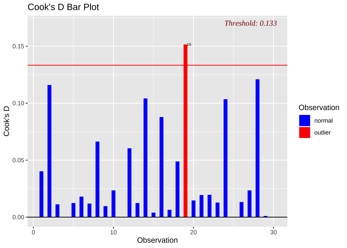
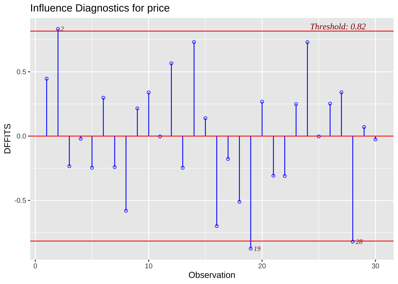
패키지 olsrr 의 함수 ols_plot_cooksd_bar 과 ols_plot_dffits 를 이용하여 각각 Cook’s distance 와 DFFIT 를 시각화할 수 있다.

ols_plot_cooksd_bar(usedcars.lm)

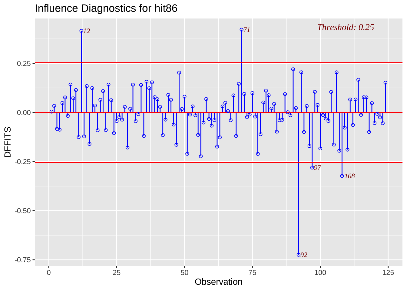
ols_plot_dffits(usedcars.lm)

L.2 교과서 연습문제 5.14

head(MLB1)

  hit85 hit86
1 0.265 0.264
2 0.309 0.296
3 0.268 0.240
4 0.243 0.229
5 0.289 0.289
6 0.266 0.286

L.2.1 회귀모형 적합

mlb1.lm <- lm(hit86 ~ hit85, data=MLB1)
summary(mlb1.lm)


Call:
lm(formula = hit86 ~ hit85, data = MLB1)

Residuals:
     Min       1Q   Median       3Q      Max 
-0.11265 -0.01708 -0.00075  0.01887  0.05700 

Coefficients:
            Estimate Std. Error t value Pr(>|t|)    
(Intercept)  0.09470    0.02310   4.100 7.49e-05 ***
hit85        0.63383    0.08622   7.351 2.47e-11 ***
---
Signif. codes:  0 '***' 0.001 '**' 0.01 '*' 0.05 '.' 0.1 ' ' 1

Residual standard error: 0.02679 on 122 degrees of freedom
Multiple R-squared:  0.307, Adjusted R-squared:  0.3013 
F-statistic: 54.04 on 1 and 122 DF,  p-value: 2.471e-11

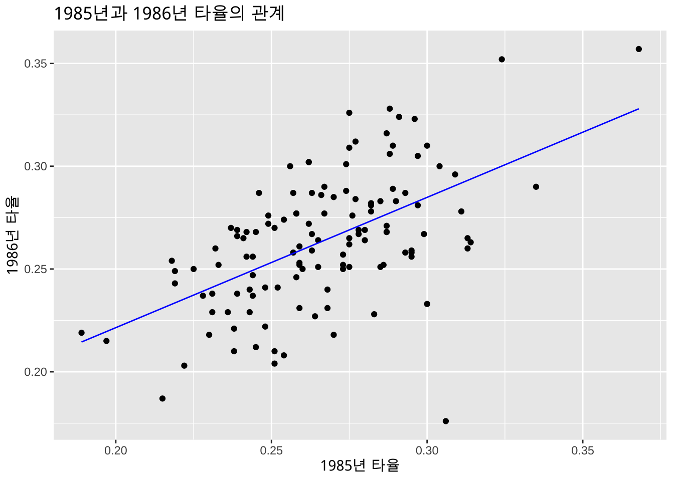
ggplot(MLB1, aes(x=hit85, y=hit86)) + geom_point() + labs(x = "1985년 타율", y = "1986년 타율") +
  labs(title="1985년과 1986년 타율의 관계") + 
  geom_line(aes(y=mlb1.lm$fitted.values), color="blue")

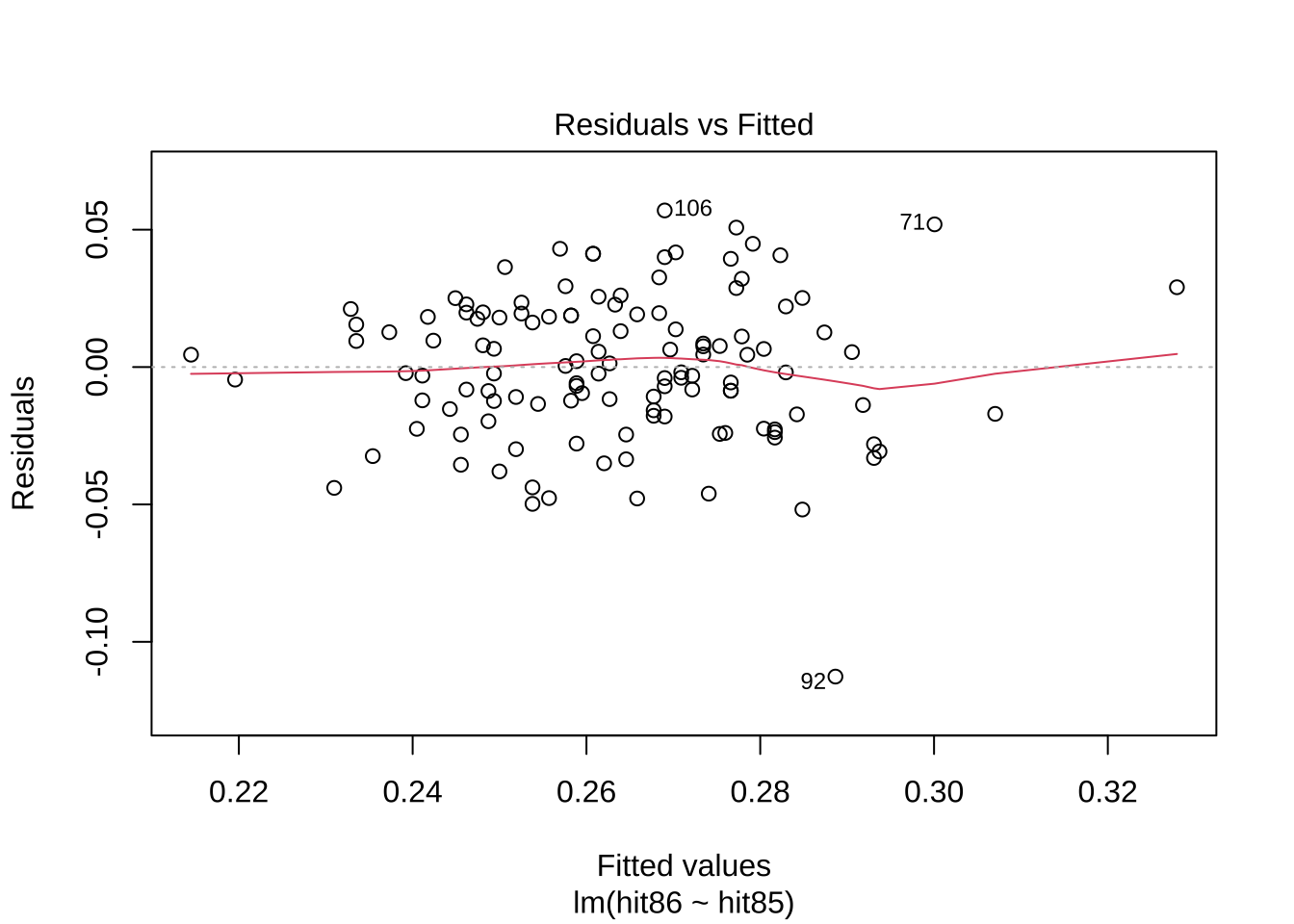
L.2.2 잔차그림

다음잔차 그림을 보면 다음과 같은 관측값이 이상점 또는 영향점일 가능성이 크다.

잔차가 큰 관측값 번호: 71, 92, 106
지렛값이 큰 관측값 번호 : 12

mlb1.lm <- lm(hit86 ~ hit85, data=MLB1)
plot(mlb1.lm)

L.2.3 잔차와 지렛값 분석

아래 잔차와 지렛값을 보면 위에서 그림을 그려서 파악한 것과 일치하는 것을 확인할 수 있다.

resid_inter <- rstandard(mlb1.lm)  # internal studentized residual
resid_exter <- rstudent(mlb1.lm)   # external studentized residual
hatval <- hatvalues(mlb1.lm)       # leverage
resid_df <- data.frame(resid_inter , resid_exter, hatval)
resid_df

    resid_inter resid_exter      hatval
1    0.05000699  0.04980213 0.008086100
2    0.20604678  0.20523630 0.026823219
3   -0.92071669 -0.92013786 0.008089609
4   -0.74122875 -0.73985250 0.013757221
5    0.41794462  0.41652651 0.013334552
6    0.85074812  0.84977870 0.008066554
7   -0.11752895 -0.11705291 0.021076586
8    1.49950517  1.50730174 0.008822848
9    0.47628862  0.47477421 0.022674209
10   1.22323441  1.22575081 0.008655952
11  -0.96655846 -0.96629590 0.016511088
12   1.15252304  1.15408980 0.114892991
13  -1.12220362 -1.12340818 0.011587908
14   0.94814587  0.94775033 0.019727886
15  -0.65464742 -0.65310705 0.056746543
16   0.94426865  0.94384613 0.017044019
17   0.29746497  0.29635083 0.014253231
18  -0.64880397 -0.64725708 0.019043095
19   0.35993460  0.35864690 0.031379027
20   0.85838160  0.85744961 0.015865556
21  -0.52346010 -0.52189678 0.028627834
22   1.54555587  1.55450230 0.008269034
23   0.60818462  0.60660721 0.010534910
24  -0.84308211 -0.84207635 0.015369379
25  -0.17556386 -0.17486494 0.058014551
26  -0.21071097 -0.20988382 0.012441433
27  -0.32339097 -0.32220100 0.012441433
28   0.24968479  0.24872294 0.013281927
29  -1.78885907 -1.80534673 0.009668354
30   0.20995888  0.20913441 0.008187340
31   1.54555587  1.55450230 0.008269034
32  -0.40887179 -0.40747191 0.011587908
33  -0.08987603 -0.08950989 0.008187340
34   1.20706156  1.20934748 0.013334552
35  -0.92405584 -0.92349840 0.016444430
36   1.61388664  1.62469547 0.009194229
37   1.08032096  1.08106766 0.012877634
38   1.36629192  1.37121192 0.012393486
39   0.47981611  0.47829711 0.025854922
40   0.68662786  0.68513312 0.009668354
41   0.28365424  0.28258253 0.010571163
42  -0.89128320 -0.89052689 0.016511088
43  -0.32339097 -0.32220100 0.012441433
44   0.74859901  0.74724285 0.014253231
45   0.71830103  0.71686860 0.008195527
46  -0.66485460 -0.66332696 0.008509772
47  -1.79282669 -1.80945914 0.008195527
48   1.53177579  1.54036942 0.017113016
49   0.17108078  0.17039863 0.010571163
50   0.65981706  0.65828292 0.014769957
51  -1.16526569 -1.16699260 0.031490124
52  -0.08849917 -0.08813855 0.013281927
53   0.28750459  0.28642092 0.011631177
54  -0.14646855 -0.14587986 0.009447831
55  -1.25801434 -1.26105391 0.008089609
56  -1.25437758 -1.25736066 0.030515312
57  -0.50371052 -0.50216434 0.010225342
58   0.73588754  0.73449735 0.008655952
59  -0.35597858 -0.35470091 0.008494569
60  -0.45705663 -0.45556979 0.021076586
61  -0.32779322 -0.32659089 0.013757221
62  -1.33805577 -1.34244750 0.016444430
63  -0.84844614 -0.84746568 0.021821186
64   0.24777624  0.24682078 0.015369379
65   0.51479711  0.51324069 0.009218787
66   0.08012340  0.07979645 0.008638411
67  -0.43719987 -0.43574587 0.008086100
68   0.95954615  0.95923199 0.008187340
69  -1.31293093 -1.31687542 0.008126362
70   0.80156331  0.80038181 0.032372217
71   1.98105733  2.00544148 0.042377621
72   0.74550574  0.74414103 0.015865556
73  -0.25726760 -0.25628058 0.008638411
74  -0.07337522 -0.07307550 0.017735660
75   0.68826166  0.68676971 0.020352702
76  -0.21977971 -0.21892046 0.008638411
77  -1.22738844 -1.22996533 0.028523754
78  -0.85364557 -0.85269021 0.016511088
79   0.36253805  0.36124383 0.019649534
80   0.83049085  0.82942806 0.017735660
81   0.97690284  0.97671857 0.008067723
82   0.16870598  0.16803274 0.013812185
83   0.48970050  0.48816941 0.008067723
84  -1.04451327 -1.04490630 0.008638411
85  -0.30800228 -0.30685670 0.015865556
86  -0.40245640 -0.40106992 0.008509772
87   0.88119841  0.88038574 0.011216193
88   0.01518447  0.01512212 0.008988241
89  -0.15011541 -0.14951273 0.008822848
90   1.90682355  1.92793919 0.012877634
91   0.23854907  0.23762483 0.009010460
92  -4.25681260 -4.59422430 0.024271666
93   1.68633876  1.69933527 0.014310534
94  -0.90035488 -0.89965120 0.012025947
95   0.32117873  0.31999502 0.010571163
96  -1.64324327 -1.65491152 0.010534910
97  -1.95470304 -1.97789425 0.019727886
98   0.58748696  0.58590363 0.031379027
99   0.42112866  0.41970434 0.008269034
100 -1.72921841 -1.74361729 0.010903785
101 -0.08361786 -0.08327684 0.023372533
102 -0.30660015 -0.30545871 0.009968065
103 -0.45847196 -0.45698295 0.008802968
104  1.10252512  1.10350851 0.008988241
105 -1.42714716 -1.43330075 0.012827348
106  2.13685857  2.16906138 0.008822848
107 -1.86838606 -1.88791915 0.010534910
108 -1.67127243 -1.68379544 0.035476081
109 -0.57561180 -0.57402789 0.017664324
110 -1.06483510 -1.06542465 0.030515312
111  0.70374907  0.70228584 0.008802968
112 -0.67499469 -0.67348138 0.008822848
113  0.70374907  0.70228584 0.008802968
114  1.47948910  1.48681148 0.012441433
115 -0.11903487 -0.11855291 0.009968065
116  0.73105151  0.72964915 0.011216193
117  0.67662401  0.67511317 0.012827348
118 -0.91392269 -0.91330116 0.011631177
119  0.17440445  0.17370986 0.070186094
120 -0.46425912 -0.46276146 0.013281927
121 -0.07146215 -0.07117016 0.009447831
122 -0.26258954 -0.26158508 0.008822848
123 -0.58988369 -0.58830072 0.008509772
124  1.56476539  1.57421623 0.009218787

resid_df %>% dplyr::arrange(desc(abs(resid_inter))) %>% head(10)

    resid_inter resid_exter      hatval
92    -4.256813   -4.594224 0.024271666
106    2.136859    2.169061 0.008822848
71     1.981057    2.005441 0.042377621
97    -1.954703   -1.977894 0.019727886
90     1.906824    1.927939 0.012877634
107   -1.868386   -1.887919 0.010534910
47    -1.792827   -1.809459 0.008195527
29    -1.788859   -1.805347 0.009668354
100   -1.729218   -1.743617 0.010903785
93     1.686339    1.699335 0.014310534

resid_df %>% dplyr::arrange(desc(hatval)) %>% head(10)

    resid_inter resid_exter     hatval
12    1.1525230   1.1540898 0.11489299
119   0.1744045   0.1737099 0.07018609
25   -0.1755639  -0.1748649 0.05801455
15   -0.6546474  -0.6531071 0.05674654
71    1.9810573   2.0054415 0.04237762
108  -1.6712724  -1.6837954 0.03547608
70    0.8015633   0.8003818 0.03237222
51   -1.1652657  -1.1669926 0.03149012
19    0.3599346   0.3586469 0.03137903
98    0.5874870   0.5859036 0.03137903

L.2.4 영향점 측도

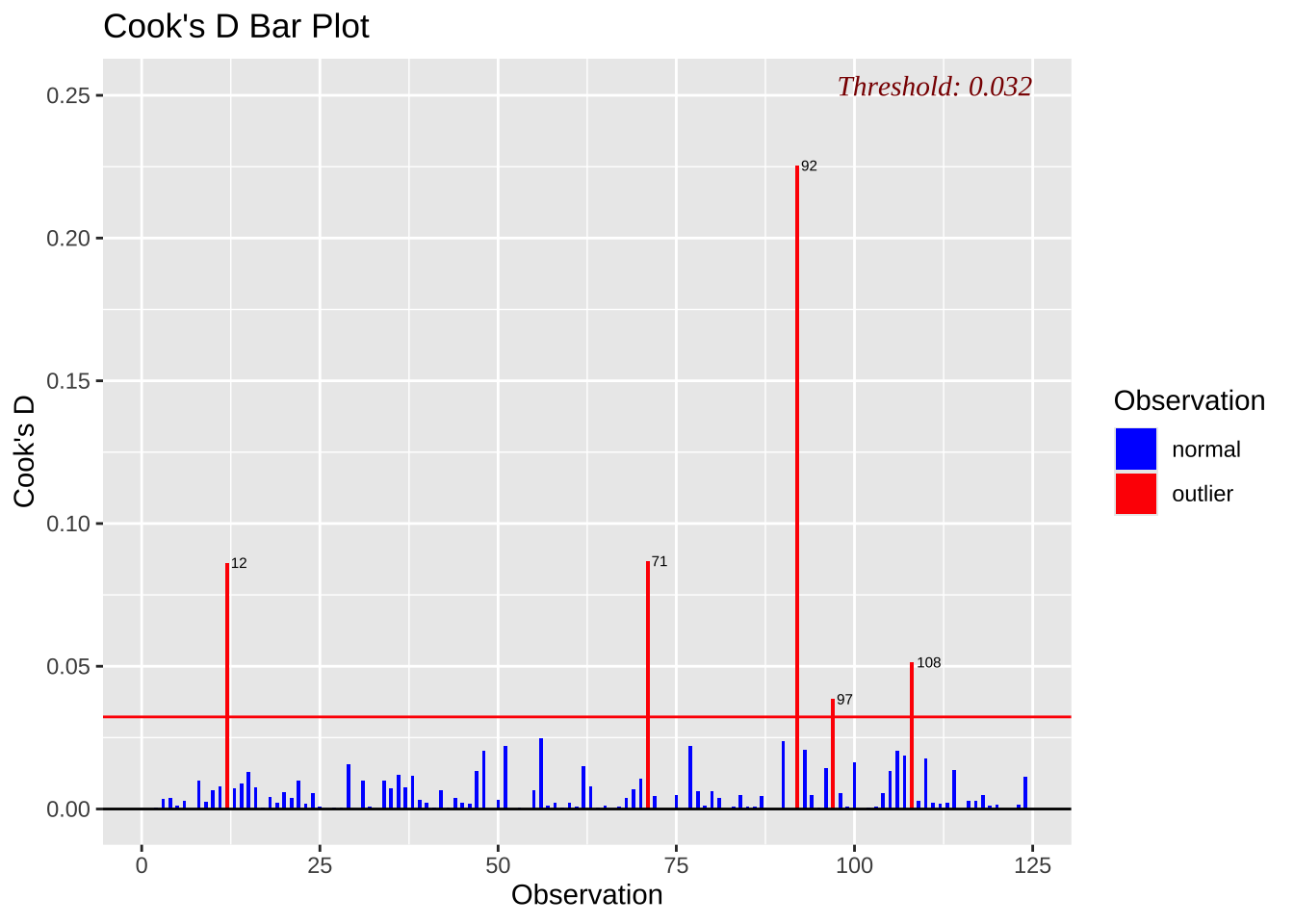
아래 COOK 거리와 DFFIT 값을 보면 다음 관측값등이 회귀 적합에 큰 영향을 미치는 것으로 나타난다.

92, 71, 12, 108, 97

위에서 잔차와 지렛값만으로 파악한 것과 거의 일치하는 것을 확인할 수 있다.

다만 차이가 나는 점은 다음과 같다.

106 번 관측값이 잔차는 매우 크지만 지렛값이 상대적으로 작아서 COOK 거리와 DFFIT 값이 크게 나타나지 않는다는 것이다.
97, 108 번 관측값은 잔차는 작지만 지렛값이 크기 때문에 COOK 거리와 DFFIT 값이 크게 나타난다는 것이다.

92, 71, 12 관측값은 잔차와 지렛값이 모두 크기 때문에 COOK 거리와 DFFIT 값이 크게 나타난다.

influence.measures(mlb1.lm)

Influence measures of
     lm(formula = hit86 ~ hit85, data = MLB1) :

       dfb.1_  dfb.ht85    dffit cov.r   cook.d     hat inf
1    0.000699 -0.000232  0.00450 1.025 1.02e-05 0.00809    
2   -0.026394  0.028494  0.03407 1.044 5.85e-04 0.02682    
3   -0.004039 -0.004628 -0.08310 1.011 3.46e-03 0.00809    
4   -0.062872  0.056210 -0.08738 1.022 3.83e-03 0.01376    
5   -0.026354  0.030441  0.04842 1.027 1.18e-03 0.01333    
6    0.009192 -0.001218  0.07663 1.013 2.94e-03 0.00807    
7   -0.014528  0.013495 -0.01718 1.038 1.49e-04 0.02108    
8   -0.027304  0.041692  0.14221 0.988 1.00e-02 0.00882    
9   -0.053240  0.058048  0.07232 1.036 2.63e-03 0.02267    
10  -0.018262  0.029939  0.11454 1.000 6.53e-03 0.00866    
11   0.079949 -0.089550 -0.12520 1.018 7.84e-03 0.01651    
12  -0.387291  0.400945  0.41580 1.124 8.62e-02 0.11489   *
13  -0.077277  0.067073 -0.12164 1.007 7.38e-03 0.01159    
14  -0.093863  0.103379  0.13445 1.022 9.05e-03 0.01973    
15   0.141276 -0.148373 -0.16019 1.070 1.29e-02 0.05675   *
16   0.098625 -0.090211  0.12429 1.019 7.73e-03 0.01704    
17   0.026146 -0.023481  0.03564 1.030 6.40e-04 0.01425    
18   0.061989 -0.068474 -0.09018 1.029 4.09e-03 0.01904    
19   0.058748 -0.055642  0.06455 1.047 2.10e-03 0.03138    
20   0.084010 -0.076341  0.10887 1.021 5.94e-03 0.01587    
21   0.070568 -0.075934 -0.08960 1.042 4.04e-03 0.02863    
22   0.036802 -0.022323  0.14195 0.985 9.96e-03 0.00827    
23   0.035849 -0.030310  0.06259 1.021 1.97e-03 0.01053    
24   0.064199 -0.072531 -0.10521 1.020 5.55e-03 0.01537    
25  -0.041733  0.040267 -0.04340 1.079 9.49e-04 0.05801   *
26   0.011921 -0.013973 -0.02356 1.029 2.80e-04 0.01244    
27   0.018301 -0.021450 -0.03616 1.028 6.59e-04 0.01244    
28   0.020330 -0.018086  0.02886 1.029 4.20e-04 0.01328    
29  -0.089226  0.072652 -0.17838 0.973 1.56e-02 0.00967    
30   0.004279 -0.002327  0.01900 1.024 1.82e-04 0.00819    
31   0.036802 -0.022323  0.14195 0.985 9.96e-03 0.00827    
32  -0.028029  0.024328 -0.04412 1.026 9.80e-04 0.01159    
33  -0.001831  0.000996 -0.00813 1.025 3.33e-05 0.00819    
34  -0.076515  0.088384  0.14059 1.006 9.85e-03 0.01333    
35  -0.093489  0.085243 -0.11941 1.019 7.14e-03 0.01644    
36   0.069829 -0.054861  0.15651 0.983 1.21e-02 0.00919    
37  -0.064901  0.075488  0.12348 1.010 7.61e-03 0.01288    
38   0.103195 -0.090783  0.15361 0.998 1.17e-02 0.01239    
39   0.068818 -0.064637  0.07792 1.040 3.06e-03 0.02585    
40   0.033861 -0.027572  0.06770 1.019 2.30e-03 0.00967    
41  -0.011489  0.014223  0.02921 1.026 4.30e-04 0.01057    
42   0.073680 -0.082528 -0.11539 1.020 6.67e-03 0.01651    
43   0.018301 -0.021450 -0.03616 1.028 6.59e-04 0.01244    
44   0.065925 -0.059208  0.08985 1.022 4.05e-03 0.01425    
45  -0.001461  0.008239  0.06517 1.016 2.13e-03 0.00820    
46   0.007749 -0.014057 -0.06145 1.018 1.90e-03 0.00851    
47   0.003689 -0.020796 -0.16448 0.972 1.33e-02 0.00820    
48  -0.132459  0.147796  0.20325 0.995 2.04e-02 0.01711    
49  -0.006928  0.008577  0.01761 1.027 1.56e-04 0.01057    
50   0.060215 -0.054307  0.08060 1.024 3.26e-03 0.01477    
51   0.169415 -0.181494 -0.21043 1.026 2.21e-02 0.03149    
52  -0.007204  0.006409 -0.01023 1.030 5.27e-05 0.01328    
53  -0.014418  0.017206  0.03107 1.027 4.86e-04 0.01163    
54   0.004051 -0.005452 -0.01425 1.026 1.02e-04 0.00945    
55  -0.005535 -0.006343 -0.11388 0.998 6.45e-03 0.00809    
56   0.178355 -0.191340 -0.22307 1.022 2.48e-02 0.03052    
57  -0.028057  0.023463 -0.05104 1.023 1.31e-03 0.01023    
58  -0.010943  0.017940  0.06863 1.016 2.36e-03 0.00866    
59  -0.010679  0.007387 -0.03283 1.023 5.43e-04 0.00849    
60  -0.056545  0.052524 -0.06685 1.035 2.25e-03 0.02108    
61  -0.027754  0.024813 -0.03857 1.029 7.49e-04 0.01376    
62  -0.135900  0.123913 -0.17358 1.003 1.50e-02 0.01644    
63  -0.107969  0.100501 -0.12658 1.027 8.03e-03 0.02182    
64  -0.018817  0.021259  0.03084 1.031 4.79e-04 0.01537    
65  -0.012600  0.017518  0.04951 1.022 1.23e-03 0.00922    
66   0.002659 -0.001920  0.00745 1.025 2.80e-05 0.00864    
67  -0.006114  0.002033 -0.03934 1.022 7.79e-04 0.00809    
68   0.019626 -0.010675  0.08715 1.010 3.80e-03 0.00819    
69  -0.022710  0.010399 -0.11920 0.996 7.06e-03 0.00813    
70   0.133778 -0.126857  0.14640 1.040 1.07e-02 0.03237    
71  -0.358382  0.379615  0.42187 0.994 8.68e-02 0.04238   *
72   0.072909 -0.066253  0.09448 1.024 4.48e-03 0.01587    
73  -0.008540  0.006166 -0.02392 1.024 2.88e-04 0.00864    
74   0.006522 -0.007251 -0.00982 1.035 4.86e-05 0.01774    
75   0.082988 -0.076917  0.09899 1.030 4.92e-03 0.02035    
76  -0.007295  0.005267 -0.02044 1.025 2.10e-04 0.00864    
77  -0.189194  0.178493 -0.21076 1.021 2.21e-02 0.02852    
78   0.070550 -0.079022 -0.11048 1.021 6.12e-03 0.01651    
79   0.042469 -0.039270  0.05114 1.035 1.32e-03 0.01965    
80  -0.074025  0.082301  0.11145 1.023 6.23e-03 0.01774    
81   0.007426  0.001756  0.08809 1.009 3.88e-03 0.00807    
82  -0.011176  0.012828  0.01989 1.030 1.99e-04 0.01381    
83   0.003712  0.000878  0.04403 1.021 9.75e-04 0.00807    
84  -0.034820  0.025141 -0.09754 1.007 4.75e-03 0.00864    
85  -0.030065  0.027320 -0.03896 1.031 7.65e-04 0.01587    
86   0.004686 -0.008499 -0.03716 1.023 6.95e-04 0.00851    
87   0.057715 -0.049704  0.09377 1.015 4.40e-03 0.01122    
88   0.000601 -0.000462  0.00144 1.026 1.05e-06 0.00899    
89   0.002708 -0.004136 -0.01411 1.025 1.00e-04 0.00882    
90  -0.115741  0.134624  0.22020 0.969 2.37e-02 0.01288    
91  -0.005069  0.007342  0.02266 1.025 2.59e-04 0.00901    
92   0.545385 -0.592108 -0.72460 0.755 2.25e-01 0.02427   *
93  -0.118528  0.135273  0.20476 0.984 2.06e-02 0.01431    
94   0.048192 -0.056968 -0.09926 1.015 4.93e-03 0.01203    
95  -0.013010  0.016106  0.03308 1.026 5.51e-04 0.01057    
96  -0.097802  0.082691 -0.17076 0.982 1.44e-02 0.01053    
97   0.195887 -0.215746 -0.28059 0.973 3.84e-02 0.01973    
98   0.095974 -0.090900  0.10546 1.044 5.59e-03 0.03138    
99   0.009936 -0.006027  0.03832 1.022 7.39e-04 0.00827    
100  0.076513 -0.093419 -0.18307 0.978 1.65e-02 0.01090    
101 -0.011158  0.010426 -0.01288 1.041 8.37e-05 0.02337    
102  0.010450 -0.013394 -0.03065 1.025 4.73e-04 0.00997    
103 -0.016699  0.012473 -0.04307 1.022 9.33e-04 0.00880    
104  0.043875 -0.033691  0.10509 1.005 5.51e-03 0.00899    
105 -0.112509  0.099557 -0.16338 0.996 1.32e-02 0.01283    
106 -0.039292  0.059996  0.20464 0.950 2.03e-02 0.00882   *
107 -0.111573  0.094334 -0.19480 0.969 1.86e-02 0.01053    
108 -0.298349  0.283857 -0.32292 1.006 5.14e-02 0.03548    
109 -0.061854  0.056746 -0.07698 1.029 2.98e-03 0.01766    
110  0.151129 -0.162132 -0.18902 1.029 1.78e-02 0.03052    
111  0.025662 -0.019169  0.06618 1.017 2.20e-03 0.00880    
112  0.012200 -0.018629 -0.06354 1.018 2.03e-03 0.00882    
113  0.025662 -0.019169  0.06618 1.017 2.20e-03 0.00880    
114 -0.084450  0.098983  0.16688 0.993 1.38e-02 0.01244    
115  0.004056 -0.005198 -0.01190 1.027 7.13e-05 0.00997    
116  0.047833 -0.041194  0.07771 1.019 3.03e-03 0.01122    
117  0.052994 -0.046894  0.07696 1.022 2.97e-03 0.01283    
118  0.045973 -0.054864 -0.09908 1.015 4.91e-03 0.01163    
119  0.046341 -0.044900  0.04773 1.093 1.15e-03 0.07019   *
120 -0.037825  0.033650 -0.05369 1.027 1.45e-03 0.01328    
121  0.001976 -0.002660 -0.00695 1.026 2.44e-05 0.00945    
122  0.004739 -0.007235 -0.02468 1.024 3.07e-04 0.00882    
123  0.006873 -0.012467 -0.05450 1.019 1.49e-03 0.00851    
124 -0.038647  0.053732  0.15185 0.985 1.14e-02 0.00922

data.frame(influence.measures(mlb1.lm)$infmat) %>% arrange(desc(cook.d)) %>% head(10)

        dfb.1_   dfb.ht85      dffit     cov.r     cook.d        hat
92   0.5453850 -0.5921082 -0.7245987 0.7553712 0.22537707 0.02427167
71  -0.3583817  0.3796146  0.4218724 0.9943835 0.08683731 0.04237762
12  -0.3872908  0.4009454  0.4158038 1.1236842 0.08621185 0.11489299
108 -0.2983494  0.2838571 -0.3229242 1.0062796 0.05136735 0.03547608
97   0.1958869 -0.2157455 -0.2805886 0.9731151 0.03844727 0.01972789
56   0.1783549 -0.1913398 -0.2230737 1.0217219 0.02476301 0.03051531
90  -0.1157414  0.1346236  0.2202043 0.9693882 0.02371680 0.01287763
77  -0.1891943  0.1784931 -0.2107561 1.0207619 0.02211610 0.02852375
51   0.1694152 -0.1814937 -0.2104279 1.0264159 0.02207447 0.03149012
93  -0.1185276  0.1352728  0.2047561 0.9838364 0.02064312 0.01431053

ols_plot_cooksd_bar(mlb1.lm)

ols_plot_dffits(mlb1.lm)

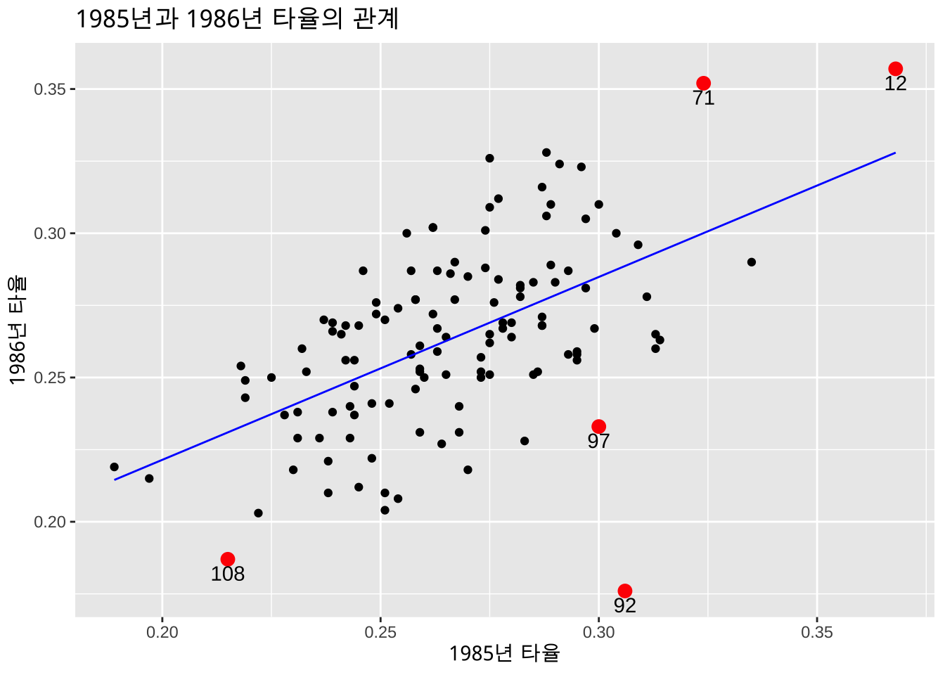
L.2.5 결론

위에서 나타난 관측값들을 나타내는 산점도를 다시 그려보자.

influnce_obs <- c(92, 71, 12, 108, 97)
MLB1$row_number <- seq_len(nrow(MLB1))

ggplot(MLB1, aes(x=hit85, y=hit86)) + geom_point() + labs(x = "1985년 타율", y = "1986년 타율") +
  labs(title="1985년과 1986년 타율의 관계") + 
  geom_line(aes(y=mlb1.lm$fitted.values), color="blue") + 
  geom_point(data = MLB1[influnce_obs, ], aes(x=hit85, y=hit86),
                    color = "red", size = 3) +
  geom_text(data = MLB1[influnce_obs, ], aes(x=hit85, y=hit86, label = row_number),
                   color = "black", vjust = 1.5, hjust = 0.5)

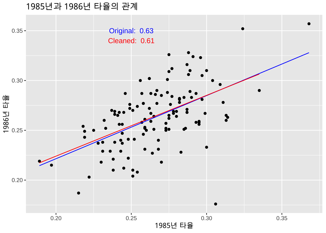
이제 영향점과 이상점을 제거한 후 회귀모형을 다시 적합해보자.

MLB1_clean <- MLB1 %>% filter(!row_number %in% influnce_obs)

mlb1_clean.lm <- lm(hit86 ~ hit85, data=MLB1_clean)
summary(mlb1_clean.lm)


Call:
lm(formula = hit86 ~ hit85, data = MLB1_clean)

Residuals:
      Min        1Q    Median        3Q       Max 
-0.051190 -0.016541 -0.000852  0.017538  0.056161 

Coefficients:
            Estimate Std. Error t value Pr(>|t|)    
(Intercept)  0.10198    0.02283   4.468 1.84e-05 ***
hit85        0.61039    0.08577   7.117 9.55e-11 ***
---
Signif. codes:  0 '***' 0.001 '**' 0.01 '*' 0.05 '.' 0.1 ' ' 1

Residual standard error: 0.02385 on 117 degrees of freedom
Multiple R-squared:  0.3021,    Adjusted R-squared:  0.2961 
F-statistic: 50.65 on 1 and 117 DF,  p-value: 9.554e-11

영향점과 이상점을 제거하기 전과 후의 회귀선을 그려서 비교해 보자.

영향점과 이상점을 제거하기 전의 기울기의 추정치는 0.633832 이다.
영향점과 이상점을 제거한 후의 기울기의 추정치는 0.6103926 이다.

p <- ggplot(MLB1, aes(x=hit85, y=hit86)) + geom_point() + labs(x = "1985년 타율", y = "1986년 타율") +
  labs(title="1985년과 1986년 타율의 관계") + 
  geom_line(aes(y=mlb1.lm$fitted.values), color="blue") + 
  geom_line(data = MLB1_clean, aes(y=mlb1_clean.lm$fitted.values), color="red") +
  #add label for two regression lines
  annotate("text", x = 0.25, y = 0.35, label = paste("Original: ", round(mlb1.lm$coef[2], 2)), color = "blue") +
  annotate("text", x = 0.25, y = 0.34, label = paste("Cleaned: ", round(mlb1_clean.lm$coef[2], 2)), color = "red")

p