AIC 와 BIC 계산
통계모형을 선택하는 척도로서 가능도함수이론에 근거한 AIC(Akaike information criteria, 식 6.9 )와 베이지안 검정이론에 기초한 BIC(bayesian or schwartz information criteria, 식 6.8 )가 있으며 정의는 모형의 선택에 대한 절에 나타니 있다.
AIC 와 BIC 는 함수 AIC 와 BIC 를 이용하면 구할 수 있다.
<- lm (price ~ ., data= houseprice)
Call:
lm(formula = price ~ ., data = houseprice)

Coefficients:
(Intercept)          tax       ground        floor         year
    1.21874      0.05195      0.01159      0.34941     -0.21894
위의 AIC 와 BIC 에서 로그 가능도 함수 \(\ell(\hat {\pmb \theta})\) 는 함수 logLik 로 구할 수 있다.
참고로 선형모형에 대한 AIC 와 BIC 는 식 6.10 에 의하여 다음과 같이 계산할 수 있다.
\[
\begin{aligned}
AIC &= n\log(2\pi) + n + n \log \frac{SSE_p}{n} + 2(p+1) \\
BIC &= n\log(2\pi) + n + n \log \frac{SSE_p}{n} + (\log n) (p+1)
\end{aligned}
\]
이제 회귀모형을 적합한 결과과 식 6.10 를 이용하여 직접 AIC 와 BIC 를 계산해보자.
<- dim (houseprice)[1 ]<- length (coef (fit1))<- deviance (fit1)c (n,p,sse)
[1] 27.00000 5.00000 91.44876
<- - 2 * logLik (fit1) + 2 * (p+ 1 )<- - 2 * logLik (fit1) + log (n)* (p+ 1 ) c (aic1, bic1)<- n* log (2 * pi) + n + n* log (deviance (fit1)/ n) + 2 * (p+ 1 ) <- n* log (2 * pi) + n + n* log (deviance (fit1)/ n) + log (n)* (p+ 1 )c (aic2, bic2)
예제 6.1
변수선택의 통계량
패키지 leaps 에 수록된 regsubsets() 함수를 이용하면 가능한 모든 모형에 대한 중요한 선택 기준들이 게산된다.
rss: 잔차 제곱합rsq: \(R^2\) adjr2 : 수정된 \(R^2\) cp : 맬로우의 \(C_p\) bic : BIC
교재 예제에 나타난 자료 houseprice는 독립변수의 수가 4개이므로 가능한 회귀식의 개수가 \(2^4=16\) 개이므로 이러한 방법을 적용할 수 있다. 하지만 독립변수의 수가 10개만 되면 가능한 회귀식의 수가 1024개나 되고 20개가 모형의 수가 100만개가 넘으므로 이들 모두에 대한 통계량을 계산하는 것은 실제로 쉽지않다.
이제 예제 자료 houseprice에 대하여 regsubsets함수를 사용하여 가능한 회귀식을 모두 적합하고 각 식에 대한 모형선택의 기준값을 계산해보자. regsubsets함수에서 nbest=6는 독립변수의 수가 같은 모형들 중에서 가장 좋은 6개의 모형만을 보여주라는 명령문이다.
모든 가능한 회귀식에 대한 통계량은 summaryf함수를 통하여 볼 수 있다.
<- regsubsets (price ~ . , data= houseprice, nbest= 6 )summaryf (houseprice.rgs)
         tax ground floor year        rss        rsq      adjr2         cp
1  ( 1 )                *       182.66315 0.86271916 0.85722792  20.943616
1  ( 2 )   *                    215.97764 0.83768158 0.83118885  28.958146
1  ( 3 )          *             628.61671 0.52756188 0.50866435 128.227503
1  ( 4 )                     * 1202.47186 0.09627993 0.06013112 266.280912
2  ( 1 )   *            *        95.19550 0.92845564 0.92249361   1.901360
2  ( 2 )                *    *  153.80917 0.88440442 0.87477146  16.002160
2  ( 3 )          *     *       168.58785 0.87329747 0.86273892  19.557496
2  ( 4 )   *      *             191.93607 0.85575007 0.84372925  25.174420
2  ( 5 )   *                 *  214.64151 0.83868576 0.82524290  30.636710
2  ( 6 )          *          *  626.80968 0.52891996 0.48966329 129.792782
3  ( 1 )   *            *    *   92.31936 0.93061720 0.92156727   3.209442
3  ( 2 )   *      *     *        93.26197 0.92990878 0.92076645   3.436208
3  ( 3 )          *     *    *  150.10029 0.88719183 0.87247773  17.109908
3  ( 4 )   *      *          *  187.51305 0.85907420 0.84069258  26.110366
4  ( 1 )   *      *     *    *   91.44876 0.93127151 0.91877542   5.000000
                bic
1  ( 1 ) -47.022941
1  ( 2 ) -42.499601
1  ( 3 ) -13.654236
1  ( 4 )   3.858312
2  ( 1 ) -61.323304
2  ( 2 ) -48.369244
2  ( 3 ) -45.892146
2  ( 4 ) -42.390102
2  ( 5 ) -39.371316
2  ( 6 ) -10.436125
3  ( 1 ) -58.855794
3  ( 2 ) -58.581513
3  ( 3 ) -45.732450
3  ( 4 ) -39.723741
4  ( 1 ) -55.815783
위의 결과를 보면 두 개의 변수 tax와 floor가 포함된 회귀식이 다음과 같은 통계량으로 가장 좋은 모형으로 나타난다.
rss: 잔차제곱합(residual sum of square), \(SSE = 95.20\) rsq: 결정계수(\(R^2_p\) ), \(R^2=0.92846\) adjr2: 수정된 결정계수(\(R^2_{ap}\) ), \(R^2_a=0.92249\) cp: 맬로우즈 \(C_p\) , \(C_p = 1.901\) bic: BIC(Bayesian Information Criteria), \(BIC= -61.323\)
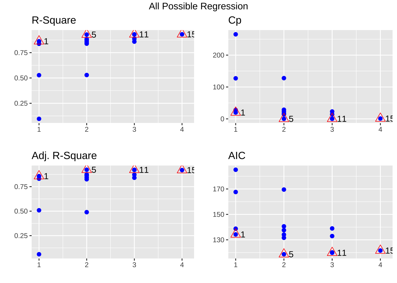
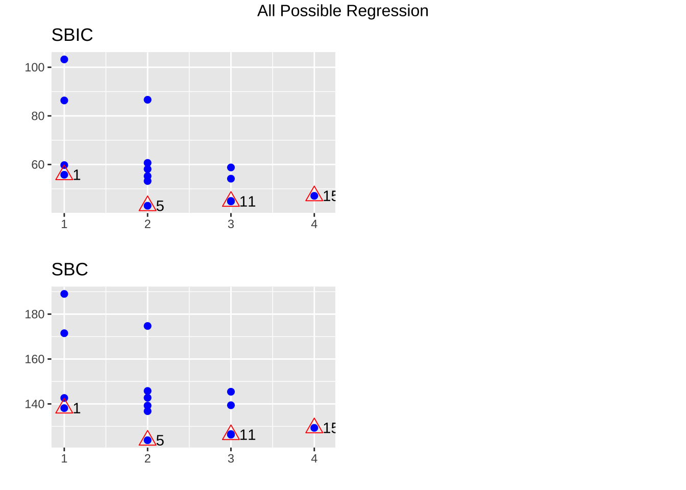
패키지 olsrr에 있는 함수 ols_step_all_possible()을 이용하면 가능한 모든 회귀모형에 대한 통계량을 구하고 여러 가지 통계량에 대한 그림을 plot() 함수를 이용하여 쉽게 그릴 수 있다.
<- lm (price ~ ., data= houseprice)<- ols_step_all_possible (fit1)
   Index N            Predictors   R-Square Adj. R-Square Mallow's Cp
3      1 1                 floor 0.86271916    0.85722792   20.943616
1      2 1                   tax 0.83768158    0.83118885   28.958146
2      3 1                ground 0.52756188    0.50866435  128.227503
4      4 1                  year 0.09627993    0.06013112  266.280912
6      5 2             tax floor 0.92845564    0.92249361    1.901360
10     6 2            floor year 0.88440442    0.87477146   16.002160
8      7 2          ground floor 0.87329747    0.86273892   19.557496
5      8 2            tax ground 0.85575007    0.84372925   25.174420
7      9 2              tax year 0.83868576    0.82524290   30.636710
9     10 2           ground year 0.52891996    0.48966329  129.792782
13    11 3        tax floor year 0.93061720    0.92156727    3.209442
11    12 3      tax ground floor 0.92990878    0.92076645    3.436208
14    13 3     ground floor year 0.88719183    0.87247773   17.109908
12    14 3       tax ground year 0.85907420    0.84069258   26.110366
15    15 4 tax ground floor year 0.93127151    0.91877542    5.000000
$ result %>% dplyr:: select (mindex, n, predictors, rsquare, adjr, cp, aic, sbc) %>% dplyr:: arrange (sbc)
   mindex n            predictors    rsquare       adjr         cp      aic
1       5 2             tax floor 0.92845564 0.92249361   1.901360 118.6453
2      11 3        tax floor year 0.93061720 0.92156727   3.209442 119.8169
3      12 3      tax ground floor 0.92990878 0.92076645   3.436208 120.0912
4      15 4 tax ground floor year 0.93127151 0.91877542   5.000000 121.5611
5       6 2            floor year 0.88440442 0.87477146  16.002160 131.5993
6       1 1                 floor 0.86271916 0.85722792  20.943616 134.2415
7       7 2          ground floor 0.87329747 0.86273892  19.557496 134.0764
8      13 3     ground floor year 0.88719183 0.87247773  17.109908 132.9403
9       2 1                   tax 0.83768158 0.83118885  28.958146 138.7648
10      8 2            tax ground 0.85575007 0.84372925  25.174420 137.5785
11     14 3       tax ground year 0.85907420 0.84069258  26.110366 138.9490
12      9 2              tax year 0.83868576 0.82524290  30.636710 140.5973
13      3 1                ground 0.52756188 0.50866435 128.227503 167.6102
14     10 2           ground year 0.52891996 0.48966329 129.792782 169.5324
15      4 1                  year 0.09627993 0.06013112 266.280912 185.1227
        sbc
1  123.8286
2  126.2961
3  126.5704
4  129.3361
5  136.7827
6  138.1290
7  139.2598
8  139.4195
9  142.6523
10 142.7618
11 145.4282
12 145.7806
13 171.4977
14 174.7158
15 189.0102
PRESS 잔차는 함수 press() 로 구할 수 있다.
\[ \text{PRESS}_p = \sum_{i=1}^n ( y_i - \hat y_{i(i)})^2 \]
또한 교과서 264 페이지에 나온 교차확인(cross validation)에 의거한 \(R^2_{pred}\) 은 다음과 같이 계산되며 press() 함수에 의해 주어진다.
\[ R^2_{pred} = 1 - \frac{ \text{PRESS}_p}{\text{SST}} \]
         tax ground floor year     PRESS pred.r.squared
1  ( 1 )                *       220.8853      0.8339932
1  ( 2 )   *                    316.0868      0.7624443
1  ( 3 )          *             838.8121      0.3695891
1  ( 4 )                     * 1430.6084      0.0000000
2  ( 1 )   *            *       144.3991      0.8914766
2  ( 2 )                *    *  207.6594      0.8439331
2  ( 3 )          *     *       233.7615      0.8243161
2  ( 4 )   *      *             358.2145      0.7307832
2  ( 5 )   *                 *  341.4294      0.7433981
2  ( 6 )          *          *  911.3553      0.3150691
3  ( 1 )   *            *    *  153.5941      0.8845661
3  ( 2 )   *      *     *       159.1752      0.8803716
3  ( 3 )          *     *    *  233.2240      0.8247200
3  ( 4 )   *      *          *  380.1744      0.7142792
4  ( 1 )   *      *     *    *  170.4810      0.8718747
이상치를 제거한 경우
교과서에서 분석하였듯이 9,10,27 번째 자료가 이상점 또는 영향점일 가능성이 높으므로 이를 제거하고 모형의 선택 기준을 다시 계산해 보자.
<- houseprice[- c (9 ,10 ,27 ),]<- lm (price ~ . , data= housepriceEX)summary (housepriceEX.lm)
Call:
lm(formula = price ~ ., data = housepriceEX)

Residuals:
    Min      1Q  Median      3Q     Max
-2.4130 -1.0459 -0.2558  0.8593  2.8197

Coefficients:
            Estimate Std. Error t value Pr(>|t|)
(Intercept)  6.32538    2.14531   2.948  0.00825 **
tax          0.06589    0.01874   3.516  0.00231 **
ground       0.00974    0.02168   0.449  0.65835
floor        0.08578    0.09057   0.947  0.35547
year        -0.11142    0.26781  -0.416  0.68205
---
Signif. codes:  0 '***' 0.001 '**' 0.01 '*' 0.05 '.' 0.1 ' ' 1

Residual standard error: 1.543 on 19 degrees of freedom
Multiple R-squared:  0.7819,    Adjusted R-squared:  0.7359
F-statistic: 17.02 on 4 and 19 DF,  p-value: 4.404e-06
이상치를 제거하면 tax 만 포함된 모형이 최적모형으로 나타난다. 이상치와 영항점이 모형의 선택에도 영향을 주는 점에 꼭 유의하자.
<- regsubsets (price ~ . , data= housepriceEX, nbest= 6 )summaryf (housepriceEX.rgs)
         tax ground floor year       rss       rsq     adjr2         cp
1  ( 1 )   *                    48.17790 0.7675502 0.7569843  0.2458362
1  ( 2 )                *      102.73566 0.5043188 0.4817878 23.1726808
1  ( 3 )          *            125.87070 0.3926964 0.3650917 32.8947363
1  ( 4 )                     * 174.34503 0.1588164 0.1205808 53.2651405
2  ( 1 )   *            *       46.18667 0.7771576 0.7559345  1.4090560
2  ( 2 )   *      *             47.39011 0.7713512 0.7495751  1.9147822
2  ( 3 )   *                 *  48.11577 0.7678500 0.7457405  2.2197243
2  ( 4 )                *    *  83.74651 0.5959380 0.5574559 17.1928590
2  ( 5 )          *     *       85.27968 0.5885408 0.5493542 17.8371405
2  ( 6 )          *          * 116.96847 0.4356480 0.3819002 31.1537464
3  ( 1 )   *      *     *       45.62514 0.7798669 0.7468469  3.1730851
3  ( 2 )   *            *    *  45.69348 0.7795371 0.7464677  3.2018056
3  ( 3 )   *      *          *  47.34784 0.7715551 0.7372884  3.8970174
3  ( 4 )          *     *    *  74.63053 0.6399210 0.5859092 15.3620431
4  ( 1 )   *      *     *    *  45.21326 0.7818541 0.7359287  5.0000000
                bic
1  ( 1 ) -28.661838
1  ( 2 ) -10.487628
1  ( 3 )  -5.613326
1  ( 4 )   2.205420
2  ( 1 ) -26.496810
2  ( 2 ) -25.879469
2  ( 3 ) -25.514758
2  ( 4 ) -12.214327
2  ( 5 ) -11.778929
2  ( 6 )  -4.195690
3  ( 1 ) -23.612331
3  ( 2 ) -23.576407
3  ( 3 ) -22.722834
3  ( 4 ) -11.802150
4  ( 1 ) -20.651921
<- ols_step_all_possible (lm (price ~ ., data= housepriceEX))$ result %>% as.data.frame () %>% dplyr:: select (mindex, n, predictors, rsquare, adjr, cp, aic, sbc) %>% dplyr:: arrange (sbc)
   mindex n            predictors   rsquare      adjr         cp       aic
1       1 1                   tax 0.7675502 0.7569843  0.2458362  90.83337
2       5 2             tax floor 0.7771576 0.7559345  1.4090560  91.82034
3       6 2            tax ground 0.7713512 0.7495751  1.9147822  92.43768
4       7 2              tax year 0.7678500 0.7457405  2.2197243  92.80240
5      11 3      tax ground floor 0.7798669 0.7468469  3.1730851  93.52677
6      12 3        tax floor year 0.7795371 0.7464677  3.2018056  93.56269
7      13 3       tax ground year 0.7715551 0.7372884  3.8970174  94.41627
8      15 4 tax ground floor year 0.7818541 0.7359287  5.0000000  95.30913
9       8 2            floor year 0.5959380 0.5574559 17.1928590 106.10283
10     14 3     ground floor year 0.6399210 0.5859092 15.3620431 105.33695
11      9 2          ground floor 0.5885408 0.5493542 17.8371405 106.53823
12      2 1                 floor 0.5043188 0.4817878 23.1726808 109.00758
13      3 1                ground 0.3926964 0.3650917 32.8947363 113.88188
14     10 2           ground year 0.4356480 0.3819002 31.1537464 114.12146
15      4 1                  year 0.1588164 0.1205808 53.2651405 121.70063
         sbc
1   94.36753
2   96.53256
3   97.14990
4   97.51461
5   99.41704
6   99.45296
7  100.30654
8  102.37745
9  110.81504
10 111.22722
11 111.25044
12 112.54174
13 117.41604
14 118.83368
15 125.23479
         tax ground floor year     PRESS pred.r.squared
1  ( 1 )   *                    56.10399     0.72930829
1  ( 2 )                *      117.36430     0.43373824
1  ( 3 )          *            157.83378     0.23848023
1  ( 4 )                     * 202.40162     0.02344834
2  ( 1 )   *            *       57.66354     0.72178375
2  ( 2 )   *      *             64.24819     0.69001399
2  ( 3 )   *                 *  63.42708     0.69397570
2  ( 4 )                *    * 108.09369     0.47846724
2  ( 5 )          *     *      114.27185     0.44865875
2  ( 6 )          *          * 160.37982     0.22619605
3  ( 1 )   *      *     *       68.98320     0.66716837
3  ( 2 )   *            *    *  65.44694     0.68423019
3  ( 3 )   *      *          *  72.26745     0.65132247
3  ( 4 )          *     *    * 109.76504     0.47040332
4  ( 1 )   *      *     *    *  79.24660     0.61764930
변수선택 방법
회귀식에서 변수를을 선택할 때 가장 큰 모형을 적합시키면 각 변수에 대한 중요도를 각 회귀계수에 대한 가설 검정 \(H_o: \beta_i=0\) 에 대한 t-통계량을 보고 판단할 수 있다.
다시 모든 자료를 고려한 houseprice에 대하여 가장 큰 모형을 적합시킨 후 각 변수에 대한 t-검정을 실시해보자.
Call:
lm(formula = price ~ ., data = houseprice)

Residuals:
    Min      1Q  Median      3Q     Max
-3.4891 -1.3574  0.1337  1.0686  3.4938

Coefficients:
            Estimate Std. Error t value Pr(>|t|)
(Intercept)  1.21874    2.04661   0.595  0.55759
tax          0.05195    0.01383   3.756  0.00109 **
ground       0.01159    0.02534   0.458  0.65169
floor        0.34941    0.07268   4.807 8.41e-05 ***
year        -0.21894    0.33149  -0.660  0.51582
---
Signif. codes:  0 '***' 0.001 '**' 0.01 '*' 0.05 '.' 0.1 ' ' 1

Residual standard error: 2.039 on 22 degrees of freedom
Multiple R-squared:  0.9313,    Adjusted R-squared:  0.9188
F-statistic: 74.53 on 4 and 22 DF,  p-value: 1.817e-12
위는 4개의 독립변수를 포함한 가장 큰 모형에 대하여 각 계수의 유의성 검정에 대한 결과이다. 변수 floor가 가장 유의한 변수이고 다음으로 tax가 유의함을 알 수 있다. 또한 2개의 변수 year와 ground는 유의하지 않음을 알 수 있다.
이렇게 독립변수들은 반응변수를 설명하는 정도가 다르므로 모든 가능한 회귀식을 적합하여 모형을 선택하는 것보다 변수의 중요도를 고려하여 변수들을 유의한 정도에 따라 차례로 모형에 포함시키거나 제거하는 절차가 더 효율적이다. 이렇게 가장 단순한 모형(평균모형)에서 시작하여 설명력이 높은 변수들을 순차적으로 포함시키거나(forward selection; 전진선택) 가장 큰 모형(full model)에서 시작하여 설명력이 낮은 변수들을 차례로 제거하는 방법(backward elimination; 후방제거)을 단계별 회귀(stepwise regression)이라고 한다.
단계별 회귀는 다음과 같은 세 가지 방법이 있다.
전진선택 (forward selection)
후방제거 (backward elimination)
단계별 선택 (stepwise selection)
단계별 선택은 전진선택과 후방제거를 결합한 형태로서 새로운 변수가 추가되는 경우마다(전진선택) 제거할 변수를 있는지 판단하여 유의하지 않다면 제거하는(후방제거) 방법이다.
단계별 선택의 적용
단계별 선택에서 전진선택과 후방제거는 add1()와 drop1()함수를 사용한다.
평균모형
\[ y=\beta_0 + \epsilon \]
<- lm (price~ 1 , houseprice)summary (model0)
Call:
lm(formula = price ~ 1, data = houseprice)

Residuals:
   Min     1Q Median     3Q    Max
-6.300 -4.275 -0.800  1.125 23.200

Coefficients:
            Estimate Std. Error t value Pr(>|t|)
(Intercept)   19.250      1.377   13.98 1.32e-13 ***
---
Signif. codes:  0 '***' 0.001 '**' 0.01 '*' 0.05 '.' 0.1 ' ' 1

Residual standard error: 7.154 on 26 degrees of freedom
첫번째 변수의 추가
이제 가장 설명력있는 변수를 추가하는데 다음과 같은 2개의 모형을 비교하는 부분 F 검정을 이용하여 가장 유의한 변수를 추가한다.
\[ H_0: y=\beta_0 + \epsilon \quad \text{vs} \quad H_1: y=\beta_0 + \beta_1 x_i + \epsilon \]
add1 (model0, scope= ~ tax+ ground+ floor+ year, test= "F" )
Single term additions

Model:
price ~ 1
       Df Sum of Sq     RSS     AIC  F value    Pr(>F)
<none>              1330.58 107.233
tax     1   1114.60  215.98  60.142 129.0183 2.310e-11 ***
ground  1    701.96  628.62  88.987  27.9170 1.792e-05 ***
floor   1   1147.92  182.66  55.619 157.1084 2.807e-12 ***
year    1    128.11 1202.47 106.500   2.6634    0.1152
---
Signif. codes:  0 '***' 0.001 '**' 0.01 '*' 0.05 '.' 0.1 ' ' 1
위의 결과에서 가장 유의한 변수가 floor이므로 회귀식에 추가한다. 변수를 추가하는 경우는 고려하는 변수를 포함한 모형과 포함하지 않는 모형이 가장 유의한 차이를 보이는 변수를 선택한다.
<- update (model0, . ~ . + floor)summary (model1)
Call:
lm(formula = price ~ floor, data = houseprice)

Residuals:
    Min      1Q  Median      3Q     Max
-4.6682 -2.1916 -0.1459  2.0517  4.9644

Coefficients:
            Estimate Std. Error t value Pr(>|t|)
(Intercept)  1.25296    1.52716    0.82     0.42
floor        0.59511    0.04748   12.53 2.81e-12 ***
---
Signif. codes:  0 '***' 0.001 '**' 0.01 '*' 0.05 '.' 0.1 ' ' 1

Residual standard error: 2.703 on 25 degrees of freedom
Multiple R-squared:  0.8627,    Adjusted R-squared:  0.8572
F-statistic: 157.1 on 1 and 25 DF,  p-value: 2.807e-12
위에서 update() 함수는 앞에서 적합한 모형 model0에 변수 floor를 추가한다.
두 번째 변수의 추가
add1 (model1, scope= ~ tax+ ground+ floor+ year, test= "F" )
Single term additions

Model:
price ~ floor
       Df Sum of Sq     RSS    AIC F value    Pr(>F)
<none>              182.663 55.619
tax     1    87.468  95.195 40.023 22.0517 8.997e-05 ***
ground  1    14.075 168.588 55.454  2.0037   0.16976
year    1    28.854 153.809 52.977  4.5023   0.04437 *
---
Signif. codes:  0 '***' 0.001 '**' 0.01 '*' 0.05 '.' 0.1 ' ' 1
<- update (model1, . ~ . + tax)summary (model2)
Call:
lm(formula = price ~ floor + tax, data = houseprice)

Residuals:
   Min     1Q Median     3Q    Max
-3.009 -1.658  0.048  1.220  3.548

Coefficients:
            Estimate Std. Error t value Pr(>|t|)
(Intercept)  0.39497    1.13994   0.346    0.732
floor        0.34835    0.06313   5.518 1.13e-05 ***
tax          0.05742    0.01223   4.696 9.00e-05 ***
---
Signif. codes:  0 '***' 0.001 '**' 0.01 '*' 0.05 '.' 0.1 ' ' 1

Residual standard error: 1.992 on 24 degrees of freedom
Multiple R-squared:  0.9285,    Adjusted R-squared:  0.9225
F-statistic: 155.7 on 2 and 24 DF,  p-value: 1.798e-14
위의 결과로부터 변수 tax가 가장 유의한 변수임을 알 수 있고 이를 모형에 추가한다.
변수의 제거
이제 독립변수가 두 개가(floor와 tax) 모형에 포함되었고 가장 최근에 포함된 변수 tax를 제외한 나머지 변수를 제거할 수 있는지 감정한다. 후방제거하는 경우는 제거할 변수가 포함된 모형과 포함하지 않는 모형의 설명력에 유의한 차이가 없어야 한다. 즉 F-검정이 유의하니 않으면 제거한다.
Single term deletions

Model:
price ~ floor + tax
       Df Sum of Sq     RSS    AIC F value    Pr(>F)
<none>               95.195 40.023
floor   1   120.782 215.978 60.142  30.451 1.126e-05 ***
tax     1    87.468 182.663 55.619  22.052 8.997e-05 ***
---
Signif. codes:  0 '***' 0.001 '**' 0.01 '*' 0.05 '.' 0.1 ' ' 1
위의 함수 drop1()의 결과에서 모든 변수에 대한 F-통계량이 유의하므로 변수를 제거하지 않는다.
세 번째 변수의 추가
독립변수가 두 개가(floor와 tax) 모형에 새로운 변수를 추가하는 검정을 실시해 보자
add1 (model2, scope= ~ tax+ ground+ floor+ year, test= "F" )
Single term additions

Model:
price ~ floor + tax
       Df Sum of Sq    RSS    AIC F value Pr(>F)
<none>              95.195 40.023
ground  1    1.9335 93.262 41.469  0.4768 0.4968
year    1    2.8761 92.319 41.194  0.7165 0.4060
위의 결과에서 유의한 변수가 없으므로 더 이상 변수를 추가하지 않는다.
최종 모형
더 이상 추가할 변수와 제거할 변수가 없으면 단계별 선택을 중단한다. 따라서 단계별 선택법에 의한 최종 모형은 floor와 tax, 두 개의 독립변수를 포함하는 모형이다.
이러한 단계별 회귀의 결과는 모든 가능한 회귀에 의한 방법과 모형이 일치한다. 독립변수의 수가 많는 경우 이러한 단계별 회귀 방법은 유용하게 사용된다.
함수 step()
위에서 논의한 세 종류의 변수선택법은 함수 step()을 이용하여 한 번에 결과를 얻을 수 있다.
주의할 점은 함수 step()은 변수의 선택 기준이 F-검정이 아니 AIC 를 이용한다는 점이다.
<- lm (price~ 1 , houseprice)step (model0, scope= ~ tax+ ground+ floor+ year, direction= "forward" )
Start:  AIC=107.23
price ~ 1

         Df Sum of Sq     RSS     AIC
+ floor   1   1147.92  182.66  55.619
+ tax     1   1114.60  215.98  60.142
+ ground  1    701.96  628.62  88.987
+ year    1    128.11 1202.47 106.500
<none>                1330.58 107.233

Step:  AIC=55.62
price ~ floor

         Df Sum of Sq     RSS    AIC
+ tax     1    87.468  95.195 40.023
+ year    1    28.854 153.809 52.977
+ ground  1    14.075 168.588 55.454
<none>                182.663 55.619

Step:  AIC=40.02
price ~ floor + tax

         Df Sum of Sq    RSS    AIC
<none>                95.195 40.023
+ year    1    2.8761 92.319 41.194
+ ground  1    1.9335 93.262 41.469
Call:
lm(formula = price ~ floor + tax, data = houseprice)

Coefficients:
(Intercept)        floor          tax
    0.39497      0.34835      0.05742
<- lm (price~ tax+ ground+ floor+ year, houseprice)step (fit, direction= "backward" )
Start:  AIC=42.94
price ~ tax + ground + floor + year

         Df Sum of Sq     RSS    AIC
- ground  1     0.871  92.319 41.194
- year    1     1.813  93.262 41.469
<none>                 91.449 42.938
- tax     1    58.652 150.100 54.318
- floor   1    96.064 187.513 60.326

Step:  AIC=41.19
price ~ tax + floor + year

        Df Sum of Sq     RSS    AIC
- year   1     2.876  95.195 40.023
<none>                92.319 41.194
- tax    1    61.490 153.809 52.977
- floor  1   122.322 214.642 61.975

Step:  AIC=40.02
price ~ tax + floor

        Df Sum of Sq     RSS    AIC
<none>                95.195 40.023
- tax    1    87.468 182.663 55.619
- floor  1   120.782 215.978 60.142
Call:
lm(formula = price ~ tax + floor, data = houseprice)

Coefficients:
(Intercept)          tax        floor
    0.39497      0.05742      0.34835
<- lm (price~ 1 , houseprice)step (model0, scope= ~ tax+ ground+ floor+ year, direction= "both" )
Start:  AIC=107.23
price ~ 1

         Df Sum of Sq     RSS     AIC
+ floor   1   1147.92  182.66  55.619
+ tax     1   1114.60  215.98  60.142
+ ground  1    701.96  628.62  88.987
+ year    1    128.11 1202.47 106.500
<none>                1330.58 107.233

Step:  AIC=55.62
price ~ floor

         Df Sum of Sq     RSS     AIC
+ tax     1     87.47   95.20  40.023
+ year    1     28.85  153.81  52.977
+ ground  1     14.08  168.59  55.454
<none>                 182.66  55.619
- floor   1   1147.92 1330.58 107.233

Step:  AIC=40.02
price ~ floor + tax

         Df Sum of Sq     RSS    AIC
<none>                 95.195 40.023
+ year    1     2.876  92.319 41.194
+ ground  1     1.934  93.262 41.469
- tax     1    87.468 182.663 55.619
- floor   1   120.782 215.978 60.142
Call:
lm(formula = price ~ floor + tax, data = houseprice)

Coefficients:
(Intercept)        floor          tax
    0.39497      0.34835      0.05742
패키지 olsrr 의 이용
패키지 olsrr 의 함수 ols_step_both_p() 이용하여 F-검정을 이용한 단계별 선택을 할 수 있다.
함수 ols_step_both_p() 이용하여 F-검정에서는 유의수준을 지정해주지 않으면 유의 수준을 0.3 으로 사용한다.
참고로 SAS 의 모형 선택에서 자동적으로 사용되는 유의수준은 전진선택에서는 0.5, 후방제거에서는 0.1 이다.
ols_step_forward_p(model, penter = 0.3,
  progress = FALSE, details = FALSE, ...)
ols_step_backward_p(model, prem = 0.3,
  progress = FALSE, details = FALSE, ...)

Forward Selection (FORWARD)

The p-values for these F statistics are compared to the SLENTRY= value that is specified in the MODEL statement (or to 0.50 if the SLENTRY= option is omitted).

Backward Elimination (BACKWARD)

F statistics significant at the SLSTAY= level specified in the MODEL statement (or at the 0.10 level if the SLSTAY= option is omitted).
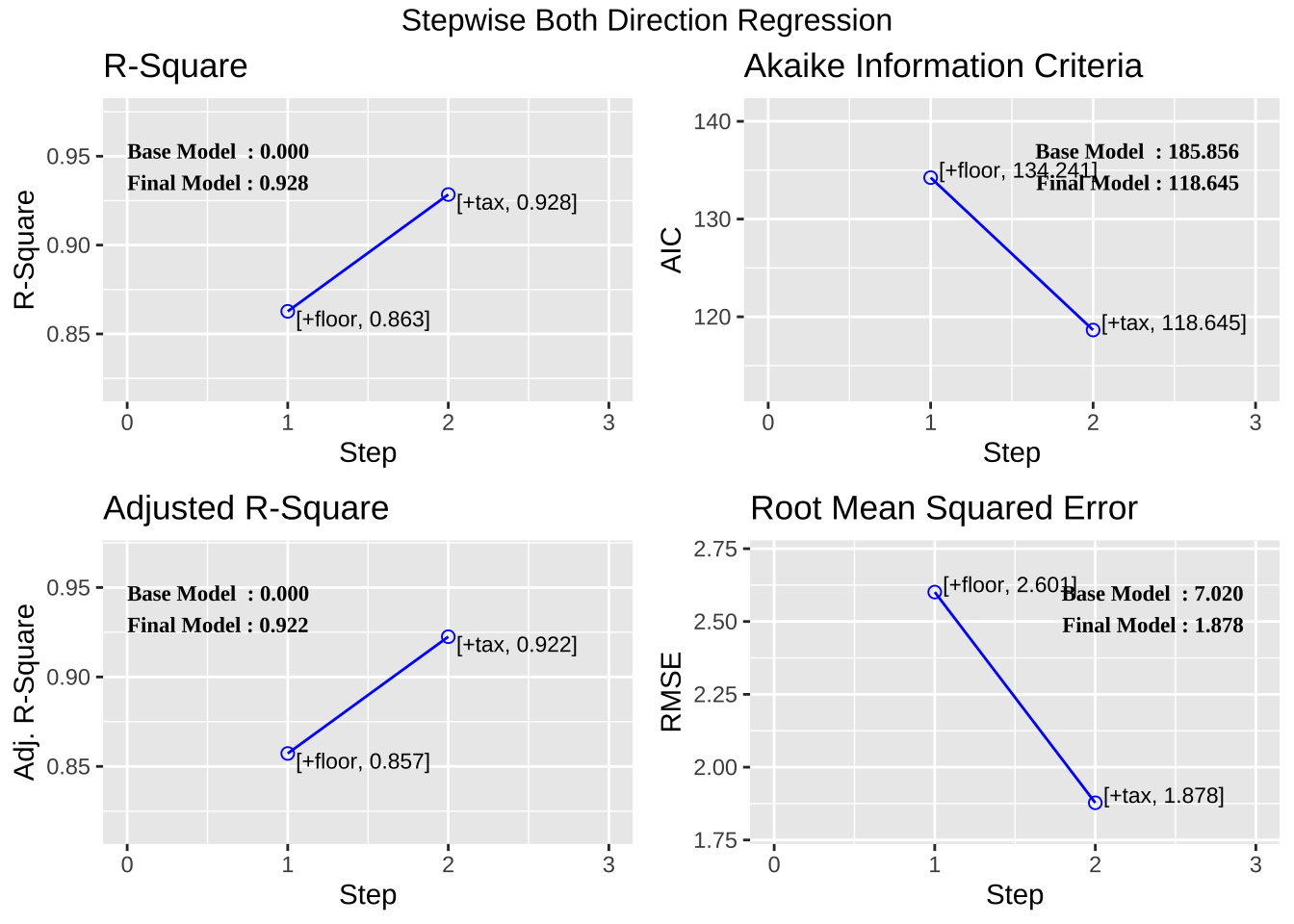
<- ols_step_both_p (fit1, details = TRUE )
Stepwise Selection Method
-------------------------

Candidate Terms:

1. tax
2. ground
3. floor
4. year


Step   => 0
Model  => price ~ 1
R2     => 0

Initiating stepwise selection...

Step      => 1
Selected  => floor
Model     => price ~ floor
R2        => 0.863

Step      => 2
Selected  => tax
Model     => price ~ floor + tax
R2        => 0.928


No more variables to be added or removed.
                             Stepwise Summary
-------------------------------------------------------------------------
Step    Variable        AIC        SBC       SBIC        R2       Adj. R2
-------------------------------------------------------------------------
 0      Base Model    185.856    188.448    105.725    0.00000    0.00000
 1      floor (+)     134.241    138.129     55.779    0.86272    0.85723
 2      tax (+)       118.645    123.829     43.032    0.92846    0.92249
-------------------------------------------------------------------------

Final Model Output
------------------

                         Model Summary
---------------------------------------------------------------
R                       0.964       RMSE                 1.878
R-Squared               0.928       MSE                  3.526
Adj. R-Squared          0.922       Coef. Var           10.346
Pred R-Squared          0.891       AIC                118.645
MAE                     1.572       SBC                123.829
---------------------------------------------------------------
 RMSE: Root Mean Square Error
 MSE: Mean Square Error
 MAE: Mean Absolute Error
 AIC: Akaike Information Criteria
 SBC: Schwarz Bayesian Criteria

                                ANOVA
---------------------------------------------------------------------
                Sum of
               Squares        DF    Mean Square       F         Sig.
---------------------------------------------------------------------
Regression    1235.385         2        617.692    155.728    0.0000
Residual        95.195        24          3.966
Total         1330.580        26
---------------------------------------------------------------------

                                 Parameter Estimates
-------------------------------------------------------------------------------------
      model     Beta    Std. Error    Std. Beta      t       Sig      lower    upper
-------------------------------------------------------------------------------------
(Intercept)    0.395         1.140                 0.346    0.732    -1.958    2.748
      floor    0.348         0.063        0.544    5.518    0.000     0.218    0.479
        tax    0.057         0.012        0.463    4.696    0.000     0.032    0.083
-------------------------------------------------------------------------------------
함수 ols_step_both_aic() 는 함수 step() 과 동일하게 AIC 를 이용하여 변수선택을 한다.
ols_step_forward_aic (fit1)
                             Stepwise Summary
-------------------------------------------------------------------------
Step    Variable        AIC        SBC       SBIC        R2       Adj. R2
-------------------------------------------------------------------------
 0      Base Model    185.856    188.448    105.725    0.00000    0.00000
 1      floor         134.241    138.129     55.779    0.86272    0.85723
 2      tax           118.645    123.829     43.032    0.92846    0.92249
-------------------------------------------------------------------------

Final Model Output
------------------

                         Model Summary
---------------------------------------------------------------
R                       0.964       RMSE                 1.878
R-Squared               0.928       MSE                  3.526
Adj. R-Squared          0.922       Coef. Var           10.346
Pred R-Squared          0.891       AIC                118.645
MAE                     1.572       SBC                123.829
---------------------------------------------------------------
 RMSE: Root Mean Square Error
 MSE: Mean Square Error
 MAE: Mean Absolute Error
 AIC: Akaike Information Criteria
 SBC: Schwarz Bayesian Criteria

                                ANOVA
---------------------------------------------------------------------
                Sum of
               Squares        DF    Mean Square       F         Sig.
---------------------------------------------------------------------
Regression    1235.385         2        617.692    155.728    0.0000
Residual        95.195        24          3.966
Total         1330.580        26
---------------------------------------------------------------------

                                 Parameter Estimates
-------------------------------------------------------------------------------------
      model     Beta    Std. Error    Std. Beta      t       Sig      lower    upper
-------------------------------------------------------------------------------------
(Intercept)    0.395         1.140                 0.346    0.732    -1.958    2.748
      floor    0.348         0.063        0.544    5.518    0.000     0.218    0.479
        tax    0.057         0.012        0.463    4.696    0.000     0.032    0.083
-------------------------------------------------------------------------------------
연습문제 6.10
자료 cars93은 1993년 미국에서 판매된 93가지 종류의 저동차에 대한 자료이다. 변수 MPG.highway를 반응변수로 하고 EngineSize, Weight, Price, Width, Length, Horsepower, Wheelbae 7개의 변수를 고려하여 가장 적합한 모형을 선택해보자.
<- Cars93[c ("MPG.highway" ,"EngineSize" , "Weight" , "Price" , "Width" , "Length" , "Horsepower" , "Wheelbase" )]head (dat93)
  MPG.highway EngineSize Weight Price Width Length Horsepower Wheelbase
1          31        1.8   2705  15.9    68    177        140       102
2          25        3.2   3560  33.9    71    195        200       115
3          26        2.8   3375  29.1    67    180        172       102
4          26        2.8   3405  37.7    70    193        172       106
5          30        3.5   3640  30.0    69    186        208       109
6          31        2.2   2880  15.7    69    189        110       105
완전모형
<- lm (MPG.highway~ . , data= dat93)summary (carfit)
Call:
lm(formula = MPG.highway ~ ., data = dat93)

Residuals:
    Min      1Q  Median      3Q     Max
-6.3952 -1.9678 -0.1942  1.4516 10.1313

Coefficients:
             Estimate Std. Error t value Pr(>|t|)
(Intercept) 21.119770  12.809426   1.649   0.1029
EngineSize   0.483792   0.698257   0.693   0.4903
Weight      -0.012833   0.001726  -7.434 7.69e-11 ***
Price       -0.047157   0.059498  -0.793   0.4302
Width        0.079770   0.228192   0.350   0.7275
Length       0.058766   0.043322   1.356   0.1785
Horsepower   0.013296   0.013443   0.989   0.3254
Wheelbase    0.277231   0.118027   2.349   0.0212 *
---
Signif. codes:  0 '***' 0.001 '**' 0.01 '*' 0.05 '.' 0.1 ' ' 1

Residual standard error: 2.95 on 85 degrees of freedom
Multiple R-squared:  0.7172,    Adjusted R-squared:  0.694
F-statistic:  30.8 on 7 and 85 DF,  p-value: < 2.2e-16
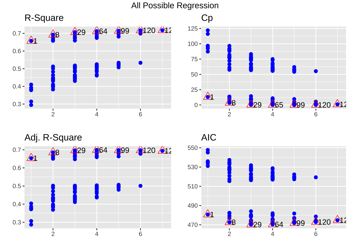
모든 가능한 회귀
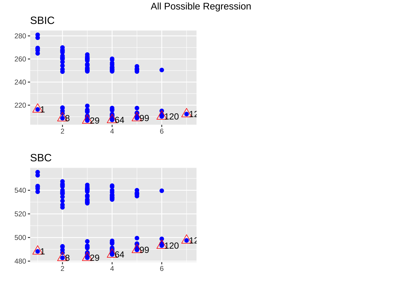
<- ols_step_all_possible (carfit)$ result %>% dplyr:: select (mindex, n, predictors, rsquare, adjr, cp, aic, sbc) %>% :: arrange (sbc) %>% head (10 )
   mindex n                         predictors   rsquare      adjr       cp
1       8 2                      Weight Length 0.6921969 0.6853568 5.527269
2       9 2                   Weight Wheelbase 0.6920227 0.6851788 5.579611
3      29 3            Weight Length Wheelbase 0.7065024 0.6966092 3.226956
4      30 3        EngineSize Weight Wheelbase 0.7045887 0.6946310 3.802229
5      31 3             Weight Width Wheelbase 0.7039881 0.6940102 3.982755
6      64 4 EngineSize Weight Length Wheelbase 0.7120588 0.6989706 3.556655
7      32 3                Weight Width Length 0.6974384 0.6872397 5.951620
8      65 4      Weight Width Length Wheelbase 0.7113915 0.6982729 3.757264
9      33 3        Weight Horsepower Wheelbase 0.6965448 0.6863160 6.220248
10     34 3           EngineSize Weight Length 0.6950183 0.6847380 6.679132
        aic      sbc
1  472.6393 482.7697
2  472.6919 482.8223
3  470.2133 482.8763
4  470.8178 483.4808
5  471.0066 483.6696
6  470.4358 485.6314
7  473.0419 485.7049
8  470.6511 485.8467
9  473.3162 485.9792
10 473.7829 486.4459
전진선택법
<- lm (MPG.highway~ 1 , data= dat93)step (model0, scope= ~ EngineSize+ Weight+ Price+ Width+ Length+ Horsepower+ Wheelbase, direction= "forward" )
Start:  AIC=312.3
MPG.highway ~ 1

             Df Sum of Sq     RSS    AIC
+ Weight      1   1718.70  896.62 214.74
+ Width       1   1072.43 1542.88 265.22
+ EngineSize  1   1027.48 1587.83 267.89
+ Horsepower  1   1002.23 1613.08 269.36
+ Wheelbase   1    990.41 1624.90 270.04
+ Price       1    822.16 1793.16 279.20
+ Length      1    770.83 1844.48 281.82
<none>                    2615.31 312.30

Step:  AIC=214.74
MPG.highway ~ Weight

             Df Sum of Sq    RSS    AIC
+ Length      1    91.615 805.00 206.72
+ Wheelbase   1    91.160 805.46 206.77
+ Width       1    53.010 843.61 211.07
+ EngineSize  1    31.068 865.55 213.46
<none>                    896.62 214.74
+ Price       1     5.845 890.77 216.13
+ Horsepower  1     2.334 894.28 216.50

Step:  AIC=206.72
MPG.highway ~ Weight + Length

             Df Sum of Sq    RSS    AIC
+ Wheelbase   1    37.413 767.59 204.29
<none>                    805.00 206.72
+ Width       1    13.708 791.29 207.12
+ EngineSize  1     7.379 797.62 207.86
+ Price       1     4.135 800.87 208.24
+ Horsepower  1     0.207 804.79 208.69

Step:  AIC=204.29
MPG.highway ~ Weight + Length + Wheelbase

             Df Sum of Sq    RSS    AIC
<none>                    767.59 204.29
+ EngineSize  1   14.5319 753.06 204.51
+ Width       1   12.7865 754.80 204.73
+ Horsepower  1    7.7950 759.79 205.34
+ Price       1    1.0351 766.55 206.16
Call:
lm(formula = MPG.highway ~ Weight + Length + Wheelbase, data = dat93)

Coefficients:
(Intercept)       Weight       Length    Wheelbase
   26.31687     -0.01107      0.08170      0.21005
후방제거
step (carfit, direction= "backward" )
Start:  AIC=208.83
MPG.highway ~ EngineSize + Weight + Price + Width + Length +
    Horsepower + Wheelbase

             Df Sum of Sq     RSS    AIC
- Width       1      1.06  740.58 206.96
- EngineSize  1      4.18  743.69 207.35
- Price       1      5.47  744.98 207.51
- Horsepower  1      8.51  748.02 207.89
- Length      1     16.01  755.52 208.82
<none>                     739.51 208.82
- Wheelbase   1     48.00  787.51 212.67
- Weight      1    480.82 1220.33 253.41

Step:  AIC=206.96
MPG.highway ~ EngineSize + Weight + Price + Length + Horsepower +
    Wheelbase

             Df Sum of Sq     RSS    AIC
- EngineSize  1      7.73  748.31 205.93
- Price       1      9.67  750.25 206.17
- Horsepower  1     10.29  750.87 206.24
<none>                     740.58 206.96
- Length      1     19.54  760.12 207.38
- Wheelbase   1     51.04  791.62 211.16
- Weight      1    514.25 1254.83 254.00

Step:  AIC=205.93
MPG.highway ~ Weight + Price + Length + Horsepower + Wheelbase

             Df Sum of Sq     RSS    AIC
- Price       1     11.48  759.79 205.34
<none>                     748.31 205.93
- Horsepower  1     18.24  766.55 206.16
- Length      1     32.26  780.57 207.85
- Wheelbase   1     51.62  799.93 210.13
- Weight      1    516.55 1264.86 252.74

Step:  AIC=205.34
MPG.highway ~ Weight + Length + Horsepower + Wheelbase

             Df Sum of Sq     RSS    AIC
- Horsepower  1      7.79  767.59 204.29
<none>                     759.79 205.34
- Length      1     33.84  793.63 207.39
- Wheelbase   1     45.00  804.79 208.69
- Weight      1    508.94 1268.73 251.03

Step:  AIC=204.29
MPG.highway ~ Weight + Length + Wheelbase

            Df Sum of Sq     RSS    AIC
<none>                    767.59 204.29
- Wheelbase  1     37.41  805.00 206.72
- Length     1     37.87  805.46 206.77
- Weight     1    846.75 1614.34 271.43
Call:
lm(formula = MPG.highway ~ Weight + Length + Wheelbase, data = dat93)

Coefficients:
(Intercept)       Weight       Length    Wheelbase
   26.31687     -0.01107      0.08170      0.21005
단계별 선택
<- lm (MPG.highway~ 1 , data= dat93)step (model0, scope= ~ EngineSize+ Weight+ Price+ Width+ Length+ Horsepower+ Wheelbase, direction= "both" )
Start:  AIC=312.3
MPG.highway ~ 1

             Df Sum of Sq     RSS    AIC
+ Weight      1   1718.70  896.62 214.74
+ Width       1   1072.43 1542.88 265.22
+ EngineSize  1   1027.48 1587.83 267.89
+ Horsepower  1   1002.23 1613.08 269.36
+ Wheelbase   1    990.41 1624.90 270.04
+ Price       1    822.16 1793.16 279.20
+ Length      1    770.83 1844.48 281.82
<none>                    2615.31 312.30

Step:  AIC=214.74
MPG.highway ~ Weight

             Df Sum of Sq     RSS    AIC
+ Length      1     91.62  805.00 206.72
+ Wheelbase   1     91.16  805.46 206.77
+ Width       1     53.01  843.61 211.07
+ EngineSize  1     31.07  865.55 213.46
<none>                     896.62 214.74
+ Price       1      5.85  890.77 216.13
+ Horsepower  1      2.33  894.28 216.50
- Weight      1   1718.70 2615.31 312.30

Step:  AIC=206.72
MPG.highway ~ Weight + Length

             Df Sum of Sq     RSS    AIC
+ Wheelbase   1     37.41  767.59 204.29
<none>                     805.00 206.72
+ Width       1     13.71  791.29 207.12
+ EngineSize  1      7.38  797.62 207.86
+ Price       1      4.14  800.87 208.24
+ Horsepower  1      0.21  804.79 208.69
- Length      1     91.62  896.62 214.74
- Weight      1   1039.48 1844.48 281.82

Step:  AIC=204.29
MPG.highway ~ Weight + Length + Wheelbase

             Df Sum of Sq     RSS    AIC
<none>                     767.59 204.29
+ EngineSize  1     14.53  753.06 204.51
+ Width       1     12.79  754.80 204.73
+ Horsepower  1      7.79  759.79 205.34
+ Price       1      1.04  766.55 206.16
- Wheelbase   1     37.41  805.00 206.72
- Length      1     37.87  805.46 206.77
- Weight      1    846.75 1614.34 271.43
Call:
lm(formula = MPG.highway ~ Weight + Length + Wheelbase, data = dat93)

Coefficients:
(Intercept)       Weight       Length    Wheelbase
   26.31687     -0.01107      0.08170      0.21005
ols_step_forward_aic (carfit, details = TRUE )
Forward Selection Method
------------------------

Candidate Terms:

1. EngineSize
2. Weight
3. Price
4. Width
5. Length
6. Horsepower
7. Wheelbase


Step     => 0
Model    => MPG.highway ~ 1
AIC      => 578.2207

Initiating stepwise selection...

                      Table: Adding New Variables
-----------------------------------------------------------------------
Predictor     DF      AIC        SBC       SBIC        R2       Adj. R2
-----------------------------------------------------------------------
Weight         1    480.663    488.261    216.331    0.65717    0.65340
Width          1    531.141    538.739    264.864    0.41006    0.40358
EngineSize     1    533.812    541.410    267.447    0.39287    0.38620
Horsepower     1    535.280    542.878    268.867    0.38322    0.37644
Wheelbase      1    535.959    543.556    269.524    0.37870    0.37187
Price          1    545.122    552.720    278.402    0.31436    0.30683
Length         1    547.746    555.344    280.948    0.29474    0.28699
-----------------------------------------------------------------------

Step     => 1
Added    => Weight
Model    => MPG.highway ~ Weight
AIC      => 480.6632

                      Table: Adding New Variables
-----------------------------------------------------------------------
Predictor     DF      AIC        SBC       SBIC        R2       Adj. R2
-----------------------------------------------------------------------
Length         1    472.639    482.770    208.747    0.69220    0.68536
Wheelbase      1    472.692    482.822    208.797    0.69202    0.68518
Width          1    476.996    487.126    212.824    0.67744    0.67027
EngineSize     1    479.384    489.514    215.061    0.66905    0.66169
Price          1    482.055    492.185    217.566    0.65940    0.65183
Horsepower     1    482.421    492.551    217.909    0.65806    0.65046
-----------------------------------------------------------------------

Step     => 2
Added    => Length
Model    => MPG.highway ~ Weight + Length
AIC      => 472.6393

                      Table: Adding New Variables
-----------------------------------------------------------------------
Predictor     DF      AIC        SBC       SBIC        R2       Adj. R2
-----------------------------------------------------------------------
Wheelbase      1    470.213    482.876    206.718    0.70650    0.69661
Width          1    473.042    485.705    209.299    0.69744    0.68724
EngineSize     1    473.783    486.446    209.975    0.69502    0.68474
Price          1    474.160    486.823    210.320    0.69378    0.68346
Horsepower     1    474.615    487.278    210.736    0.69228    0.68190
-----------------------------------------------------------------------

Step     => 3
Added    => Wheelbase
Model    => MPG.highway ~ Weight + Length + Wheelbase
AIC      => 470.2133

                      Table: Adding New Variables
-----------------------------------------------------------------------
Predictor     DF      AIC        SBC       SBIC        R2       Adj. R2
-----------------------------------------------------------------------
EngineSize     1    470.436    485.631    207.247    0.71206    0.69897
Width          1    470.651    485.847    207.438    0.71139    0.69827
Horsepower     1    471.264    486.460    207.982    0.70948    0.69628
Price          1    472.088    487.283    208.714    0.70690    0.69358
-----------------------------------------------------------------------


No more variables to be added.

Variables Selected:

=> Weight
=> Length
=> Wheelbase
                             Stepwise Summary
-------------------------------------------------------------------------
Step    Variable        AIC        SBC       SBIC        R2       Adj. R2
-------------------------------------------------------------------------
 0      Base Model    578.221    583.286    311.963    0.00000    0.00000
 1      Weight        480.663    488.261    216.331    0.65717    0.65340
 2      Length        472.639    482.770    208.747    0.69220    0.68536
 3      Wheelbase     470.213    482.876    206.718    0.70650    0.69661
-------------------------------------------------------------------------

Final Model Output
------------------

                         Model Summary
---------------------------------------------------------------
R                       0.841       RMSE                 2.873
R-Squared               0.707       MSE                  8.254
Adj. R-Squared          0.697       Coef. Var           10.097
Pred R-Squared          0.665       AIC                470.213
MAE                     2.139       SBC                482.876
---------------------------------------------------------------
 RMSE: Root Mean Square Error
 MSE: Mean Square Error
 MAE: Mean Absolute Error
 AIC: Akaike Information Criteria
 SBC: Schwarz Bayesian Criteria

                               ANOVA
--------------------------------------------------------------------
                Sum of
               Squares        DF    Mean Square      F         Sig.
--------------------------------------------------------------------
Regression    1847.724         3        615.908    71.413    0.0000
Residual       767.588        89          8.625
Total         2615.312        92
--------------------------------------------------------------------

                                  Parameter Estimates
----------------------------------------------------------------------------------------
      model      Beta    Std. Error    Std. Beta      t        Sig      lower     upper
----------------------------------------------------------------------------------------
(Intercept)    26.317         7.088                  3.713    0.000    12.233    40.401
     Weight    -0.011         0.001       -1.225    -9.909    0.000    -0.013    -0.009
     Length     0.082         0.039        0.224     2.095    0.039     0.004     0.159
  Wheelbase     0.210         0.101        0.269     2.083    0.040     0.010     0.410
----------------------------------------------------------------------------------------
ols_step_forward_p (carfit, details = TRUE )
Forward Selection Method
------------------------

Candidate Terms:

1. EngineSize
2. Weight
3. Price
4. Width
5. Length
6. Horsepower
7. Wheelbase


Step   => 0
Model  => MPG.highway ~ 1
R2     => 0

Initiating stepwise selection...

                    Selection Metrics Table
----------------------------------------------------------------
Predictor     Pr(>|t|)    R-Squared    Adj. R-Squared      AIC
----------------------------------------------------------------
Weight         0.00000        0.657             0.653    480.663
Width          0.00000        0.410             0.404    531.141
EngineSize     0.00000        0.393             0.386    533.812
Horsepower     0.00000        0.383             0.376    535.280
Wheelbase      0.00000        0.379             0.372    535.959
Price          0.00000        0.314             0.307    545.122
Length         0.00000        0.295             0.287    547.746
----------------------------------------------------------------

Step      => 1
Selected  => Weight
Model     => MPG.highway ~ Weight
R2        => 0.657

                    Selection Metrics Table
----------------------------------------------------------------
Predictor     Pr(>|t|)    R-Squared    Adj. R-Squared      AIC
----------------------------------------------------------------
Length         0.00190        0.692             0.685    472.639
Wheelbase      0.00195        0.692             0.685    472.692
Width          0.01952        0.677             0.670    476.996
EngineSize     0.07563        0.669             0.662    479.384
Price          0.44422        0.659             0.652    482.055
Horsepower     0.62912        0.658             0.650    482.421
----------------------------------------------------------------

Step      => 2
Selected  => Length
Model     => MPG.highway ~ Weight + Length
R2        => 0.692

                    Selection Metrics Table
----------------------------------------------------------------
Predictor     Pr(>|t|)    R-Squared    Adj. R-Squared      AIC
----------------------------------------------------------------
Wheelbase      0.04014        0.707             0.697    470.213
Width          0.21761        0.697             0.687    473.042
EngineSize     0.36665        0.695             0.685    473.783
Price          0.49960        0.694             0.683    474.160
Horsepower     0.88015        0.692             0.682    474.615
----------------------------------------------------------------

Step      => 3
Selected  => Wheelbase
Model     => MPG.highway ~ Weight + Length + Wheelbase
R2        => 0.707

                    Selection Metrics Table
----------------------------------------------------------------
Predictor     Pr(>|t|)    R-Squared    Adj. R-Squared      AIC
----------------------------------------------------------------
EngineSize     0.19593        0.712             0.699    470.436
Width          0.22536        0.711             0.698    470.651
Horsepower     0.34463        0.709             0.696    471.264
Price          0.73113        0.707             0.694    472.088
----------------------------------------------------------------

Step      => 4
Selected  => EngineSize
Model     => MPG.highway ~ Weight + Length + Wheelbase + EngineSize
R2        => 0.712

                    Selection Metrics Table
----------------------------------------------------------------
Predictor     Pr(>|t|)    R-Squared    Adj. R-Squared      AIC
----------------------------------------------------------------
Width          0.46764        0.714             0.697    471.869
Horsepower     0.56977        0.713             0.697    472.088
Price          0.61570        0.713             0.696    472.165
----------------------------------------------------------------


No more variables to be added.

Variables Selected:

=> Weight
=> Length
=> Wheelbase
=> EngineSize
                             Stepwise Summary
-------------------------------------------------------------------------
Step    Variable        AIC        SBC       SBIC        R2       Adj. R2
-------------------------------------------------------------------------
 0      Base Model    578.221    583.286    311.963    0.00000    0.00000
 1      Weight        480.663    488.261    216.331    0.65717    0.65340
 2      Length        472.639    482.770    208.747    0.69220    0.68536
 3      Wheelbase     470.213    482.876    206.718    0.70650    0.69661
 4      EngineSize    470.436    485.631    207.247    0.71206    0.69897
-------------------------------------------------------------------------

Final Model Output
------------------

                         Model Summary
---------------------------------------------------------------
R                       0.844       RMSE                 2.846
R-Squared               0.712       MSE                  8.097
Adj. R-Squared          0.699       Coef. Var           10.057
Pred R-Squared          0.664       AIC                470.436
MAE                     2.081       SBC                485.631
---------------------------------------------------------------
 RMSE: Root Mean Square Error
 MSE: Mean Square Error
 MAE: Mean Absolute Error
 AIC: Akaike Information Criteria
 SBC: Schwarz Bayesian Criteria

                               ANOVA
--------------------------------------------------------------------
                Sum of
               Squares        DF    Mean Square      F         Sig.
--------------------------------------------------------------------
Regression    1862.256         4        465.564    54.404    0.0000
Residual       753.056        88          8.557
Total         2615.312        92
--------------------------------------------------------------------

                                  Parameter Estimates
----------------------------------------------------------------------------------------
      model      Beta    Std. Error    Std. Beta      t        Sig      lower     upper
----------------------------------------------------------------------------------------
(Intercept)    28.439         7.246                  3.925    0.000    14.040    42.839
     Weight    -0.012         0.001       -1.334    -8.960    0.000    -0.015    -0.009
     Length     0.063         0.041        0.172     1.511    0.134    -0.020     0.145
  Wheelbase     0.233         0.102        0.298     2.282    0.025     0.030     0.435
 EngineSize     0.766         0.587        0.149     1.303    0.196    -0.402     1.933
----------------------------------------------------------------------------------------
연습문제 6.12
set.seed (13111 )<- 10 <- 50 <- 100 <- (num_of_ind_var+ 1 )* n<- matrix (rnorm (N), ncol= num_of_ind_var+ 1 )<- data.frame (randata)<- names (randata)[1 : 50 ]<- NULL <- NULL <- NULL <- NULL for (i in 1 : Nsim) {<- matrix (rnorm (N), ncol= num_of_ind_var+ 1 )<- data.frame (randata)# === 함수 step(..direction="backward")는 AIC 를 이용 <- lm (X51 ~ ., data= randata)<- step (fit.lm, direction= "backward" , trace= 0 )<- as.character (attr (res$ terms, "variables" ))[- c (1 ,2 )]# ==== 함수 step(...direction = "forward"..) 은 AIC 를 이용 # fit.null <- lm(X51 ~ 1, data=randata) # res <- step(fit.null, scope~ X1 + X2 + X3 + X4 + X5 + X6 + X7 + X8 + X9 + X10 + X11 + X12 + # X13 + X14 + X15 + X16 + X17 + X18 + X19 + X20 + X21 + X22 + # X23 + X24 + X25 + X26 + X27 + X28 + X29 + X30 + X31 + X32 + # X33 + X34 + X35 + X36 + X37 + X38 + X39 + X40 + X41 + X42 + # X43 + X44 + X45 + X46 + X47 + X48 + X49 + X50 , direction = "forward", trace=0) # ariable.entered <- as.character(attr(res$terms, "variables"))[-c(1,2)] # === 함수 ols_step_backward_p 는 F-검정을 이용 # fit.lm <- lm(X51 ~ ., data=randata) # aa <- ols_step_backward_p(fit.lm) # variable.entered <- names(aa$model$coefficients)[-1] # === 함수 ols_step_forward_p 는 F-검정을 이용 # fit.lm <- lm(X51 ~ ., data=randata) # aa <- ols_step_forward_p(fit.lm) # variable.entered <- names(aa$model$coefficients)[-1] <- c (variables.set, variable.entered )<- c (p, length (variable.entered))<- c ( r2.set , summary (res)$ r.squared)<- c ( r2adj.set , summary (res)$ adj.r.squared)<- factor (variables.set, levels= indvarname)table (variables.set)
variables.set
 X1  X2  X3  X4  X5  X6  X7  X8  X9 X10 X11 X12 X13 X14 X15 X16 X17 X18 X19 X20
  2   3   3   3   2   5   5   1   5   0   3   4   0   4   2   4   3   2   1   2
X21 X22 X23 X24 X25 X26 X27 X28 X29 X30 X31 X32 X33 X34 X35 X36 X37 X38 X39 X40
  6   3   4   2   4   4   3   1   4   3   2   3   2   1   3   4   2   1   2   5
X41 X42 X43 X44 X45 X46 X47 X48 X49 X50
  2   2   3   2   2   3   1   2   4   0
   Min. 1st Qu.  Median    Mean 3rd Qu.    Max.
    7.0     9.0    14.0    13.4    17.0    20.0
   Min. 1st Qu.  Median    Mean 3rd Qu.    Max.
 0.2228  0.2909  0.3612  0.3570  0.4050  0.5094
   Min. 1st Qu.  Median    Mean 3rd Qu.    Max.
 0.1545  0.2094  0.2635  0.2595  0.2938  0.3852